Statistical Analysis
Lab 7: T-Tests, Choropleth Maps, and Correlations
Bogdan G. Popescu 
John Cabot University
A Basic World Map
Choropleth Map: Life Expectancy
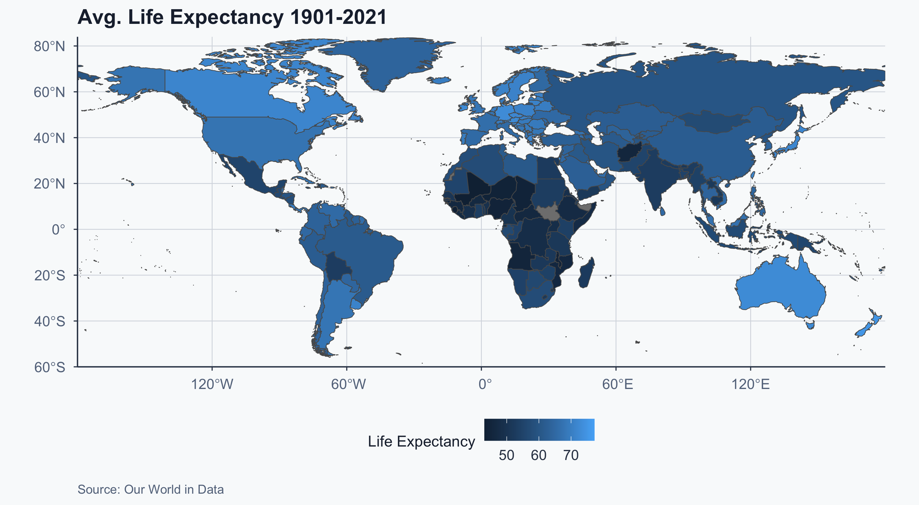
Improved Choropleth
Show code
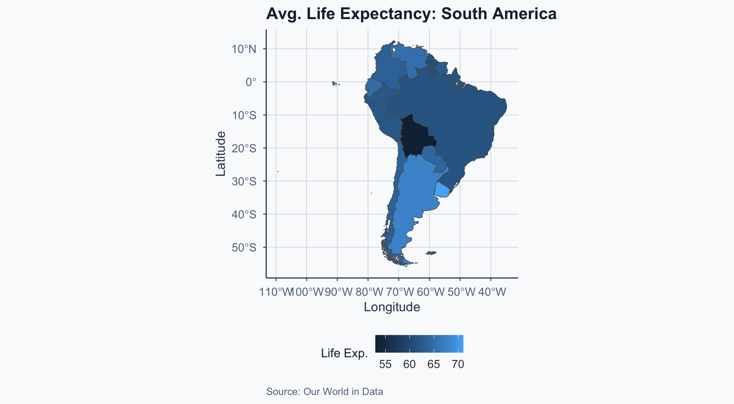
Map: South America
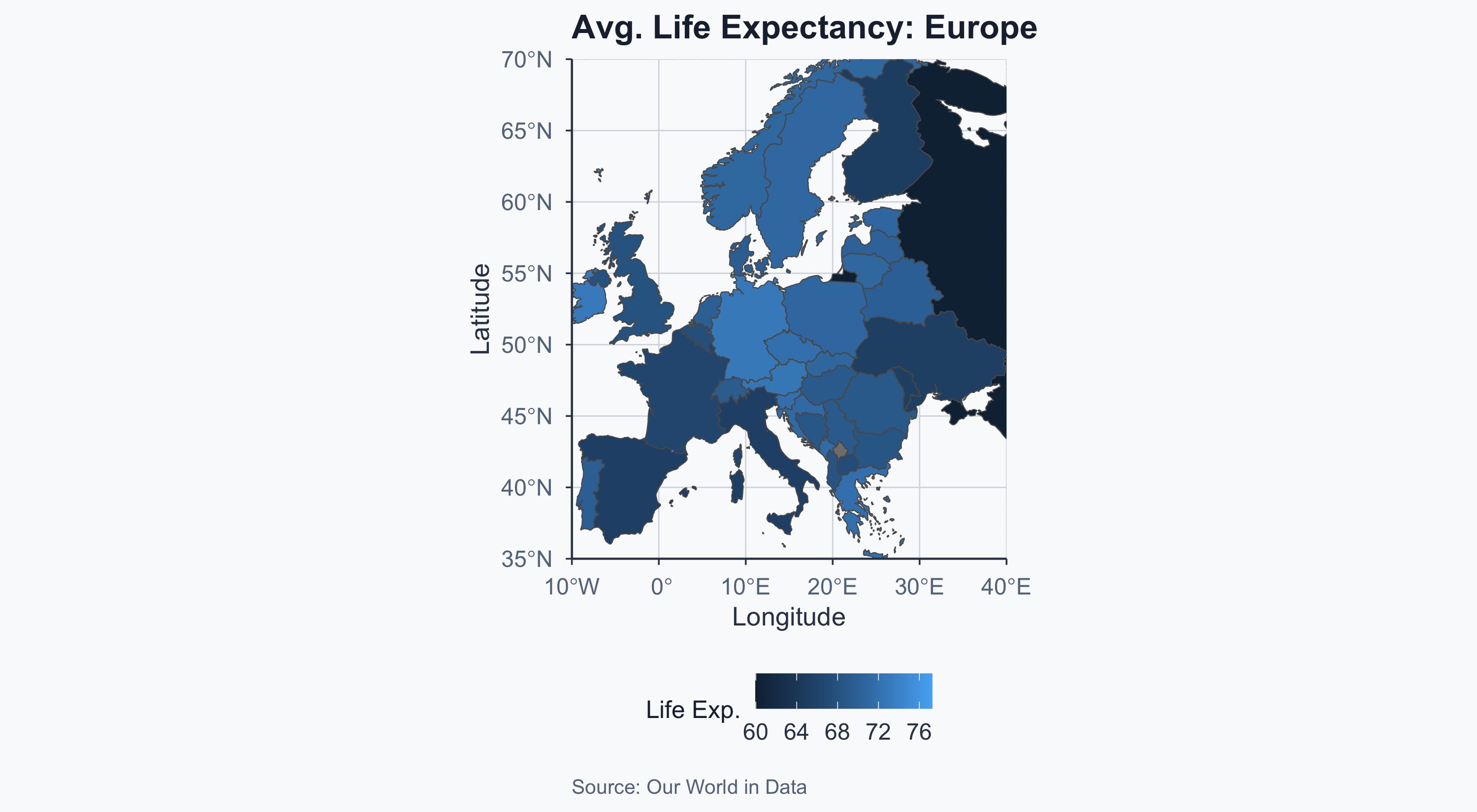
Map: Europe
Boxplot: Latam vs EU
Show code
box_dat <- rbind(sample_latam, sample_eu)

ggplot(box_dat, aes(
  x = continent, y = life_exp_mean, color = continent
)) +
  geom_boxplot(linewidth = 0.8) +
  coord_cartesian(xlim = c(0, 3), ylim = c(40, 80)) +
  scale_color_manual(values = c(
    "Europe" = sage, "South America" = gold
  )) +
  labs(
    title = "Life Expectancy: South America vs Europe",
    x = "", y = "Life Expectancy",
    caption = "Source: Our World in Data"
  ) +
  theme_meridian() +
  theme(legend.position = "none")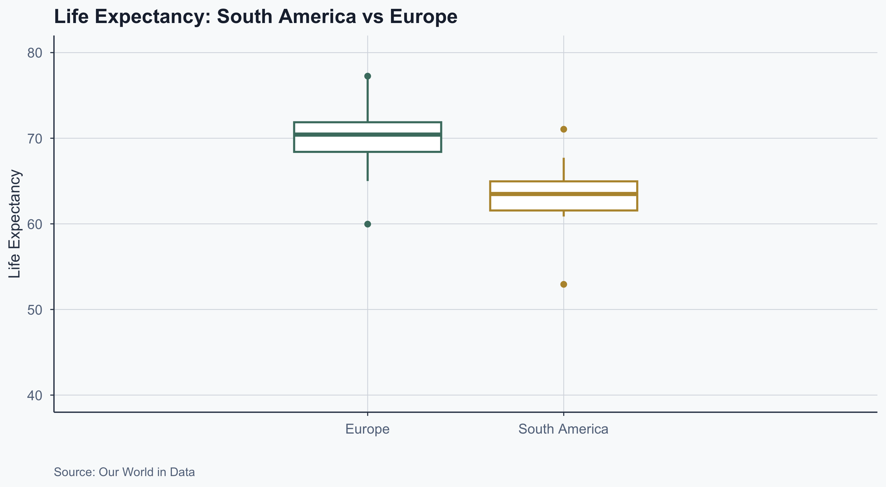
Interpreting a Boxplot
Show code
merged_latam_bp <- subset(box_dat, continent == "South America")
hwy_50 <- quantile(merged_latam_bp$life_exp_mean, 0.5)
hwy_25 <- quantile(merged_latam_bp$life_exp_mean, 0.25)
hwy_75 <- quantile(merged_latam_bp$life_exp_mean, 0.75)
sd_bp <- sd(merged_latam_bp$life_exp_mean, na.rm = TRUE) / 4
hwy_iqr <- hwy_75 - hwy_25

merged_eu_bp <- subset(box_dat, continent == "Europe")
hwy2_25 <- quantile(merged_eu_bp$life_exp_mean, 0.25, na.rm = TRUE)
hwy2_75 <- quantile(merged_eu_bp$life_exp_mean, 0.75, na.rm = TRUE)
hwy2_min <- boxplot.stats(merged_eu_bp$life_exp_mean)$stats[1]
hwy2_max <- boxplot.stats(merged_eu_bp$life_exp_mean)$stats[5]

outliermax <- max(merged_latam_bp$life_exp_mean, na.rm = TRUE)
outliermin <- min(merged_latam_bp$life_exp_mean, na.rm = TRUE)

ggplot(box_dat, aes(
  x = continent, y = life_exp_mean, color = continent
)) +
  geom_boxplot() +
  coord_cartesian(xlim = c(0, 3), ylim = c(40, 80)) +
  scale_color_manual(values = c(
    "Europe" = sage, "South America" = gold
  )) +
  annotate("text", y = hwy_50 - sd_bp, x = 2,
           label = "Median", color = terracotta, fontface = 2) +
  annotate("text", y = hwy_25 - 1, x = 3,
           label = "25th percentile", color = terracotta, fontface = 3) +
  annotate("segment", y = hwy_25, yend = hwy_25,
           x = 2.6, xend = 2.4, color = terracotta,
           arrow = arrow(length = unit(0.3, "lines"))) +
  annotate("text", y = hwy_75 + 1, x = 3,
           label = "75th percentile", color = terracotta, fontface = 3) +
  annotate("segment", y = hwy_75, yend = hwy_75,
           x = 2.6, xend = 2.4, color = terracotta,
           arrow = arrow(length = unit(0.3, "lines"))) +
  annotate("text", y = hwy_25 + 2 * hwy_iqr, x = -0.1,
           label = "Interquartile\n range (IQR)", color = sage) +
  annotate("segment", y = c(hwy2_25, hwy2_75),
           yend = c(hwy2_25, hwy2_75), color = sage,
           x = 0.2, xend = 0.6,
           arrow = arrow(length = unit(0.3, "lines"))) +
  annotate("segment", y = hwy2_25, yend = hwy2_75,
           x = 0.2, xend = 0.2, color = sage) +
  annotate("text", y = hwy2_max, x = 0.8,
           label = "Maximum\n75% + (1.5 \u00d7 IQR)",
           hjust = 1, lineheight = 1, color = sage) +
  annotate("segment", y = hwy2_max, yend = hwy2_max,
           x = 1, xend = 0.8, color = sage,
           arrow = arrow(length = unit(0.3, "lines"))) +
  annotate("text", y = hwy2_min, x = 0.8,
           label = "Minimum\n25% - (1.5 \u00d7 IQR)",
           hjust = 1, lineheight = 1, color = sage) +
  annotate("segment", y = hwy2_min, yend = hwy2_min,
           x = 1, xend = 0.8, color = sage,
           arrow = arrow(length = unit(0.3, "lines"))) +
  annotate("text", y = outliermax, x = 2.3,
           label = "Outlier", color = terracotta, fontface = 2) +
  annotate("text", y = outliermin, x = 2.3,
           label = "Outlier", color = terracotta, fontface = 2) +
  labs(
    title = "Anatomy of a Boxplot",
    x = "", y = "Life Expectancy",
    caption = "Source: Our World in Data"
  ) +
  theme_meridian() +
  theme(legend.position = "none")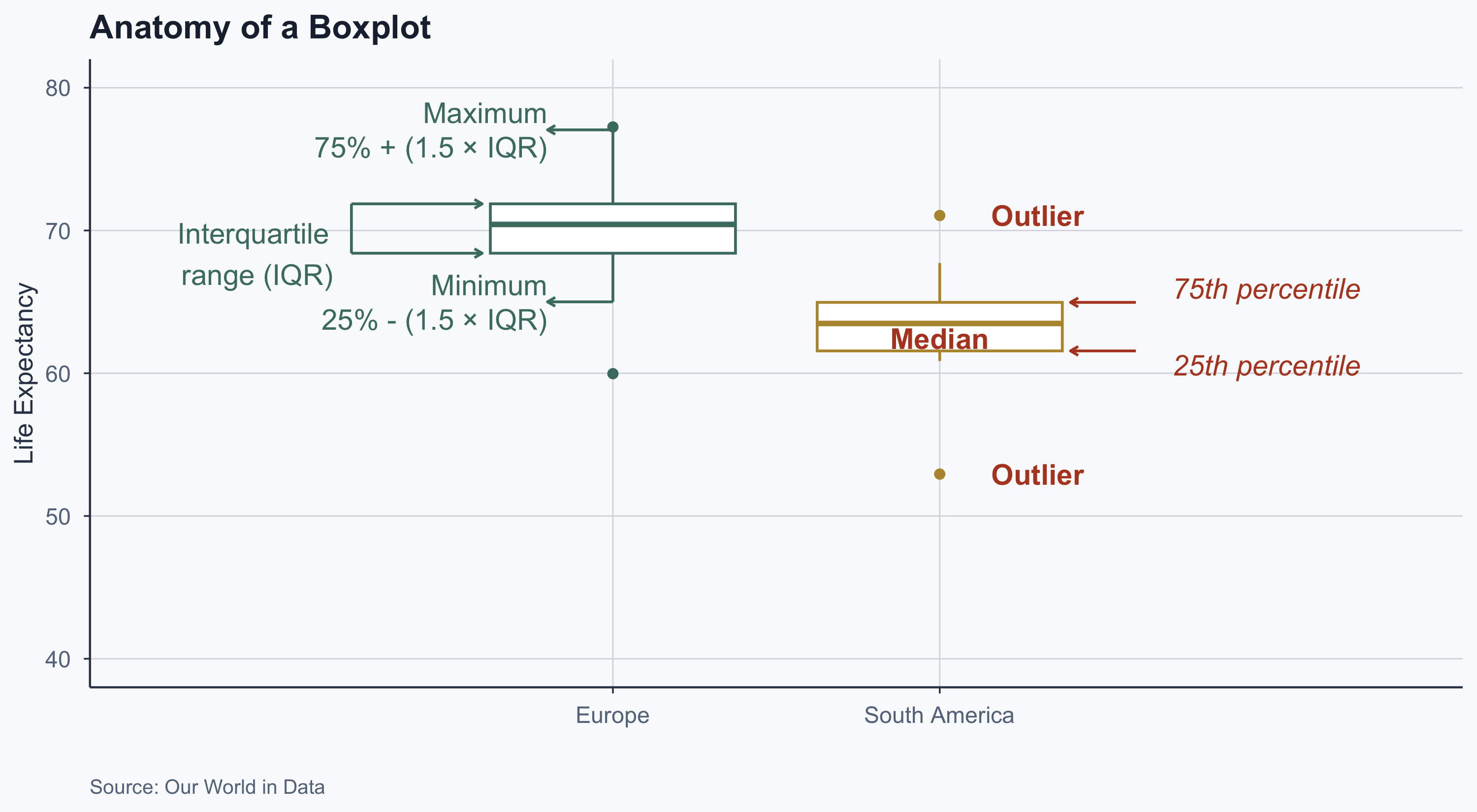
Boxplot with Jitter
Adding individual observations with geom_jitter:
Show code
ggplot(box_dat, aes(
  x = continent, y = life_exp_mean, color = continent
)) +
  geom_boxplot(linewidth = 0.8) +
  geom_jitter(width = 0.15, alpha = 0.6) +
  scale_color_manual(values = c(
    "Europe" = sage, "South America" = gold
  )) +
  labs(
    title = "Life Expectancy with Individual Countries",
    x = "", y = "Life Expectancy",
    caption = "Source: Our World in Data"
  ) +
  theme_meridian() +
  theme(legend.position = "none")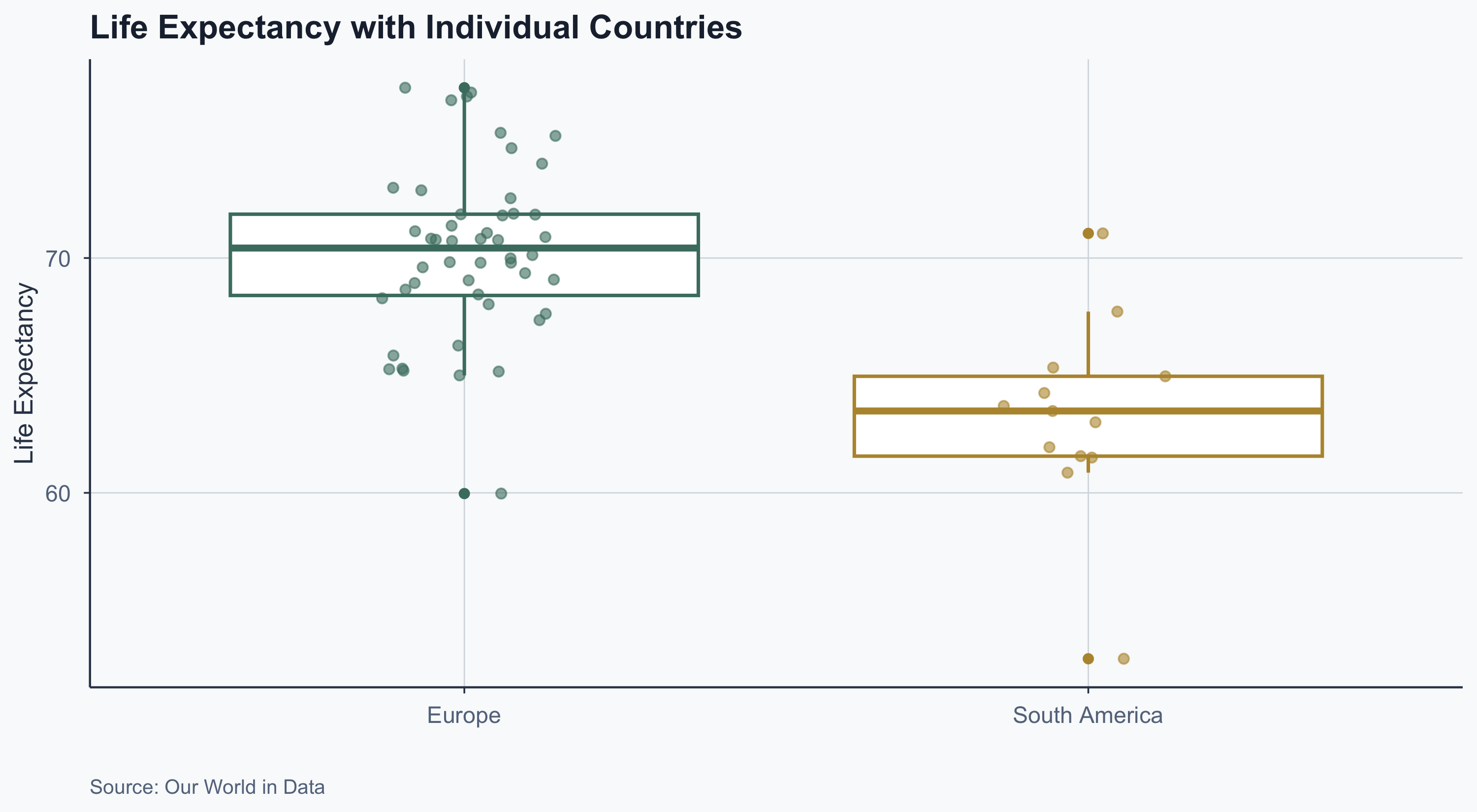
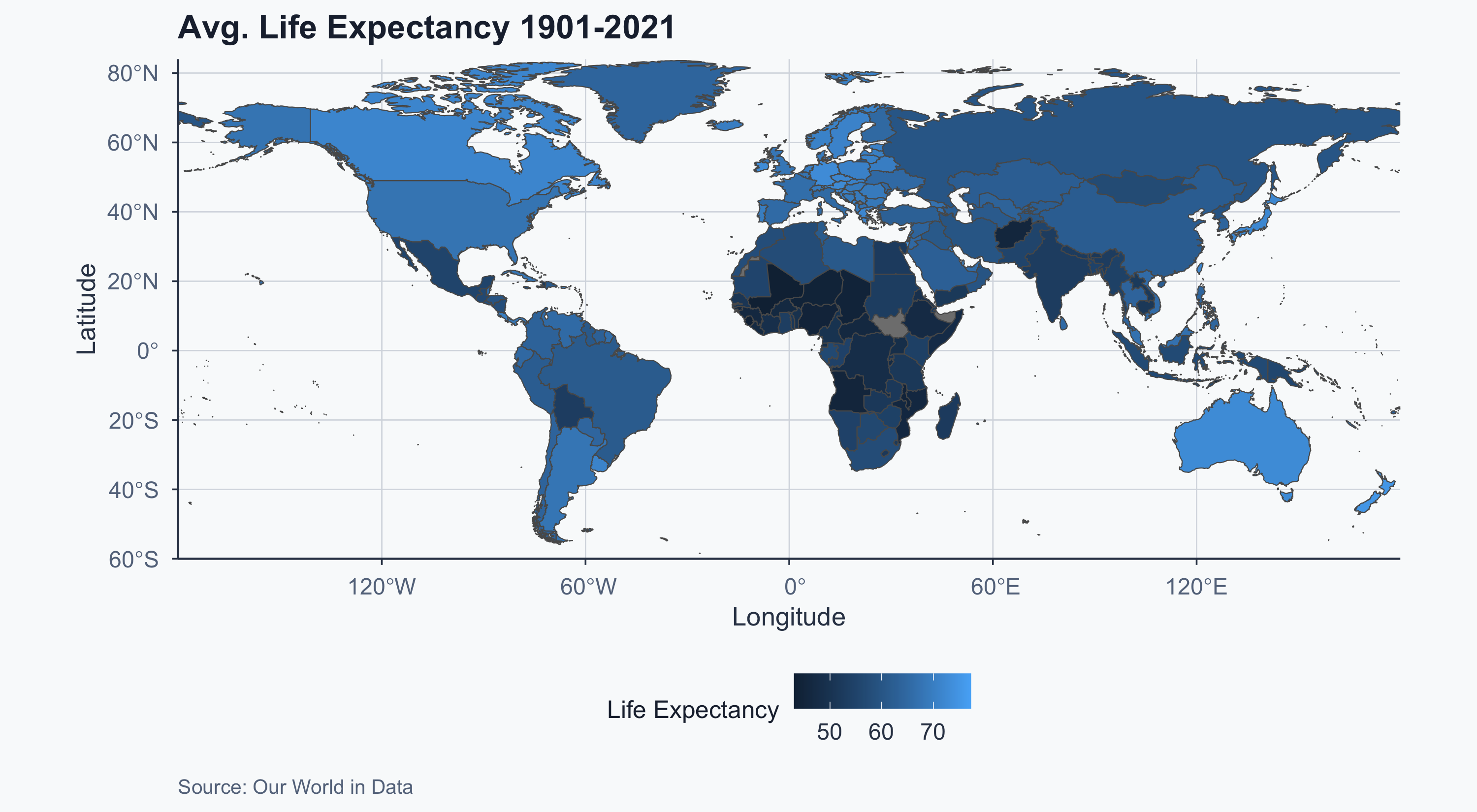
Europe: Average Life Expectancy
Show code
ggplot() +
  geom_sf(data = box_dat, aes(fill = life_exp_mean)) +
  coord_sf(
    xlim = c(min_lon_x, max_lon_x),
    ylim = c(min_lat_y, max_lat_y),
    expand = FALSE
  ) +
  labs(
    title = "Avg. Life Expectancy 1901-2021",
    x = "Longitude", y = "Latitude",
    fill = "Life Exp.",
    caption = "Source: Our World in Data"
  ) +
  theme_meridian()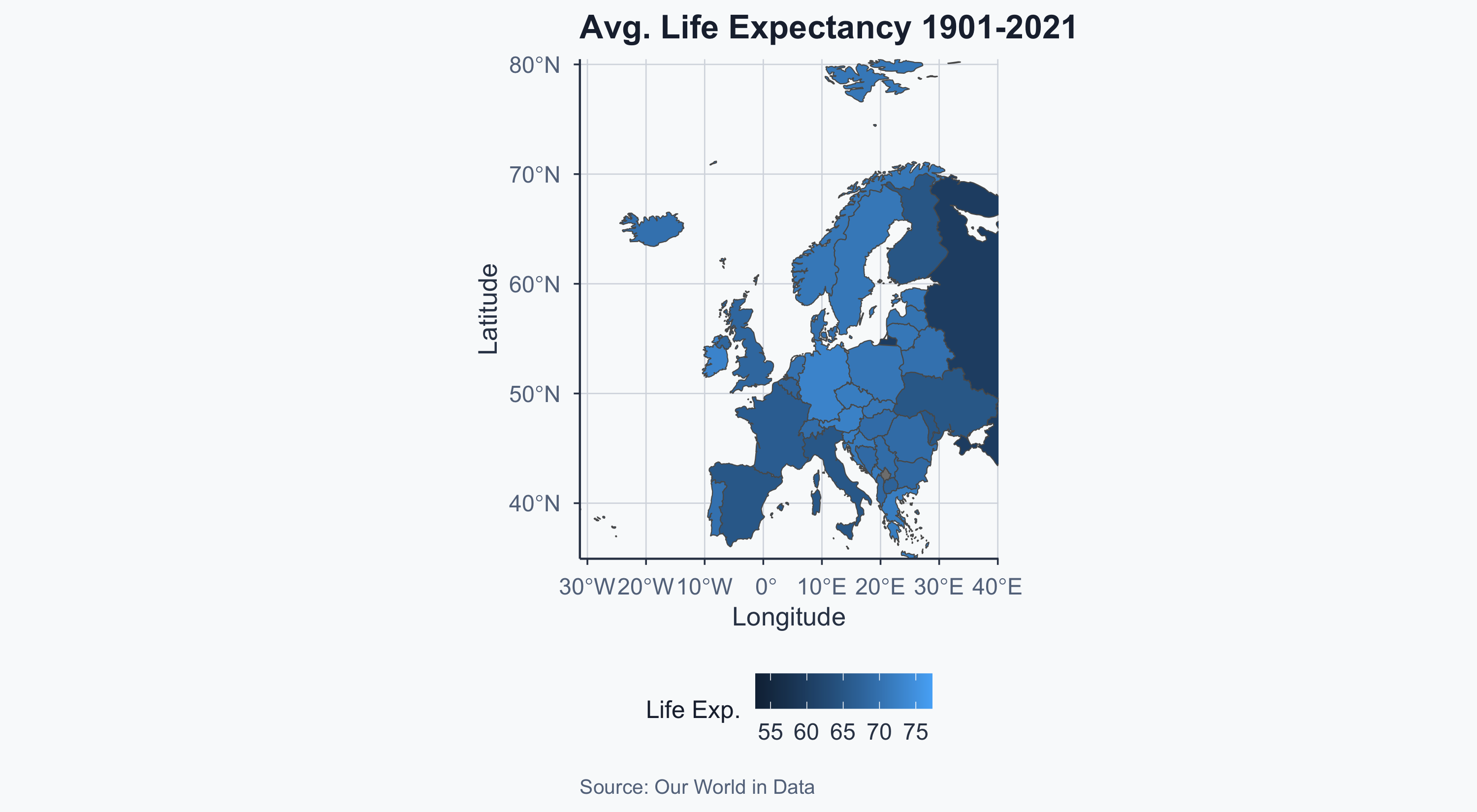
Visualizing the Boundary Points
Show code
euro_extreme <- data.frame(
  x_lon = c(min_lon_x, max_lon_x, min_lon_x, max_lon_x),
  y_lat = c(min_lat_y, max_lat_y, max_lat_y, min_lat_y),
  name = c("South-West", "North-East", "North-West", "South-East")
)

ggplot() +
  geom_sf(data = box_dat, aes(fill = life_exp_mean)) +
  geom_point(
    data = euro_extreme, aes(x = x_lon, y = y_lat),
    fill = "blue", color = "darkred", size = 3
  ) +
  geom_label_repel(
    data = euro_extreme,
    aes(x = x_lon, y = y_lat, label = name),
    fill = alpha("white", 0.8)
  ) +
  coord_sf(
    xlim = c(min_lon_x - 3, max_lon_x + 3),
    ylim = c(min_lat_y - 3, max_lat_y + 3),
    expand = FALSE
  ) +
  labs(
    title = "Avg. Life Expectancy with Boundary Points",
    x = "Longitude", y = "Latitude",
    fill = "Life Exp.",
    caption = "Source: Our World in Data"
  ) +
  theme_meridian()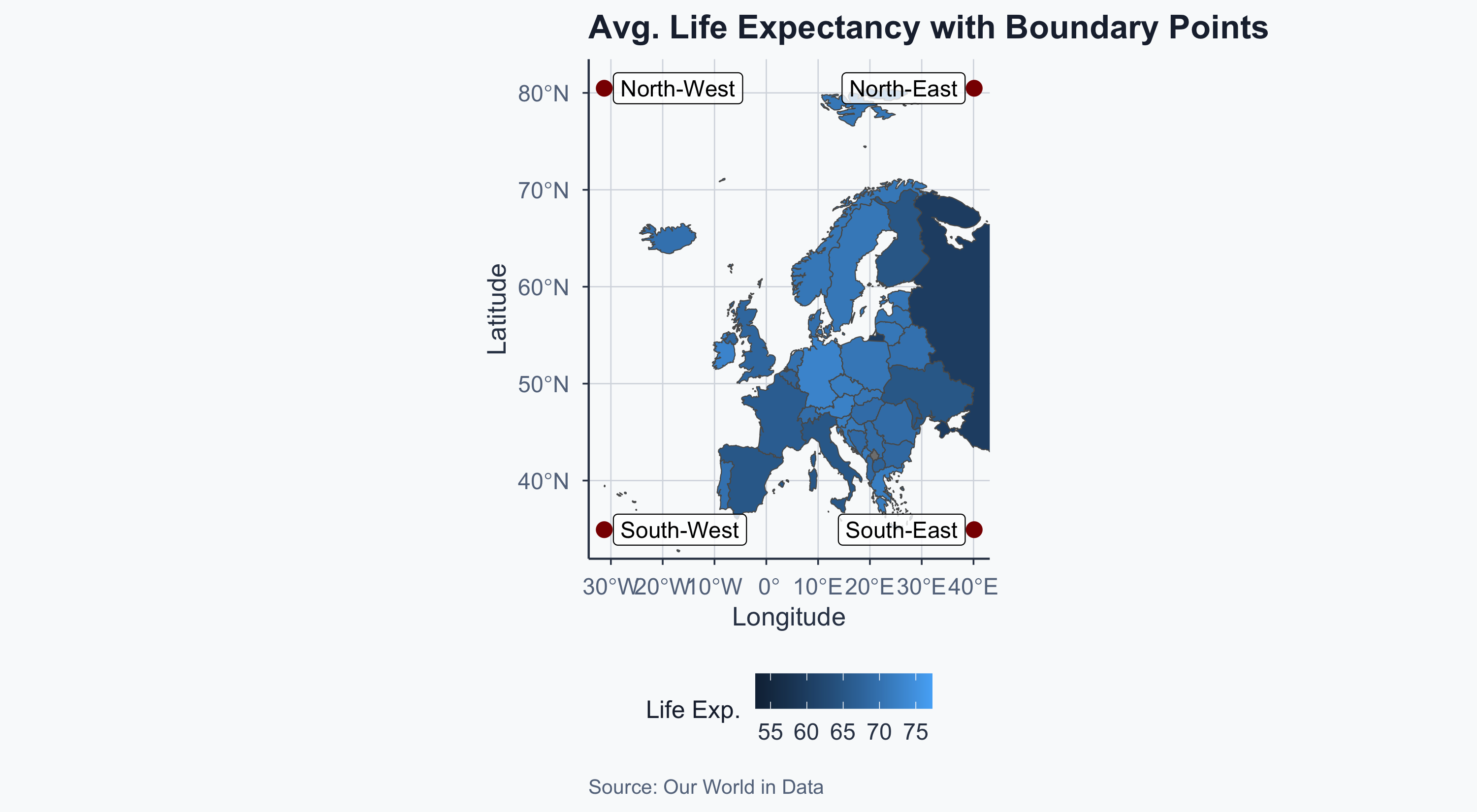
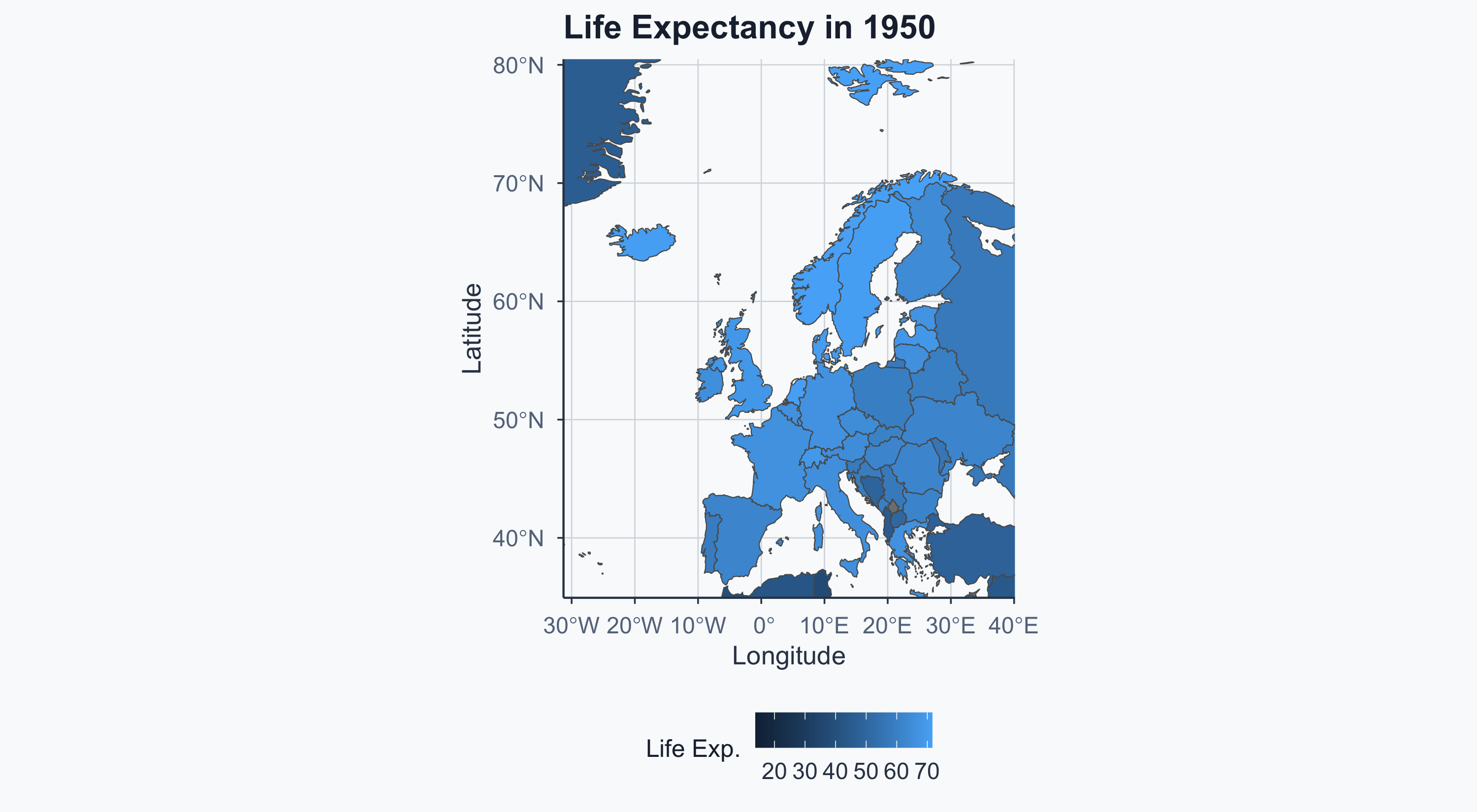
Map: Europe 1950
Show code
Map: Europe 2020
Show code
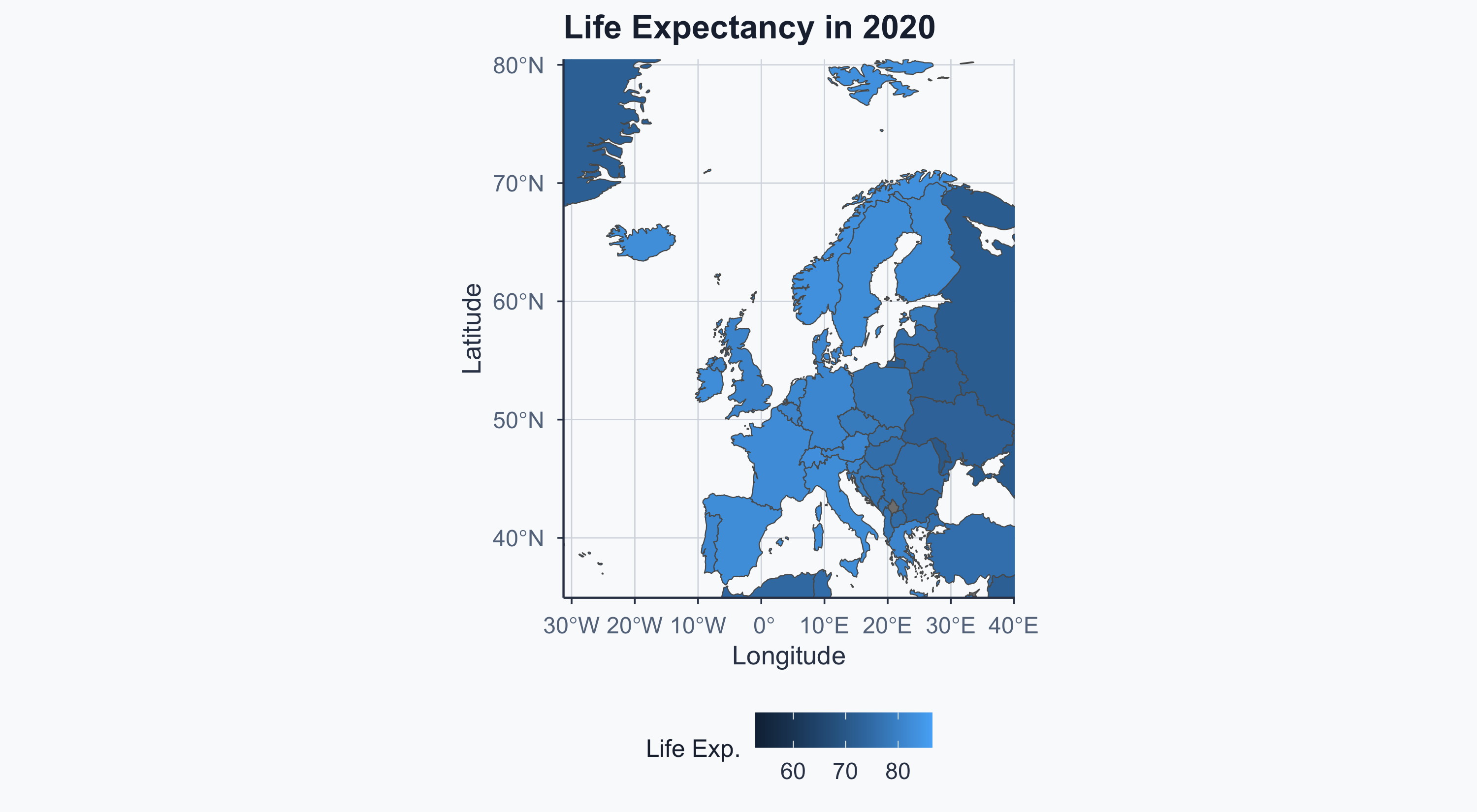
Side by Side (Without Fixed Scale)
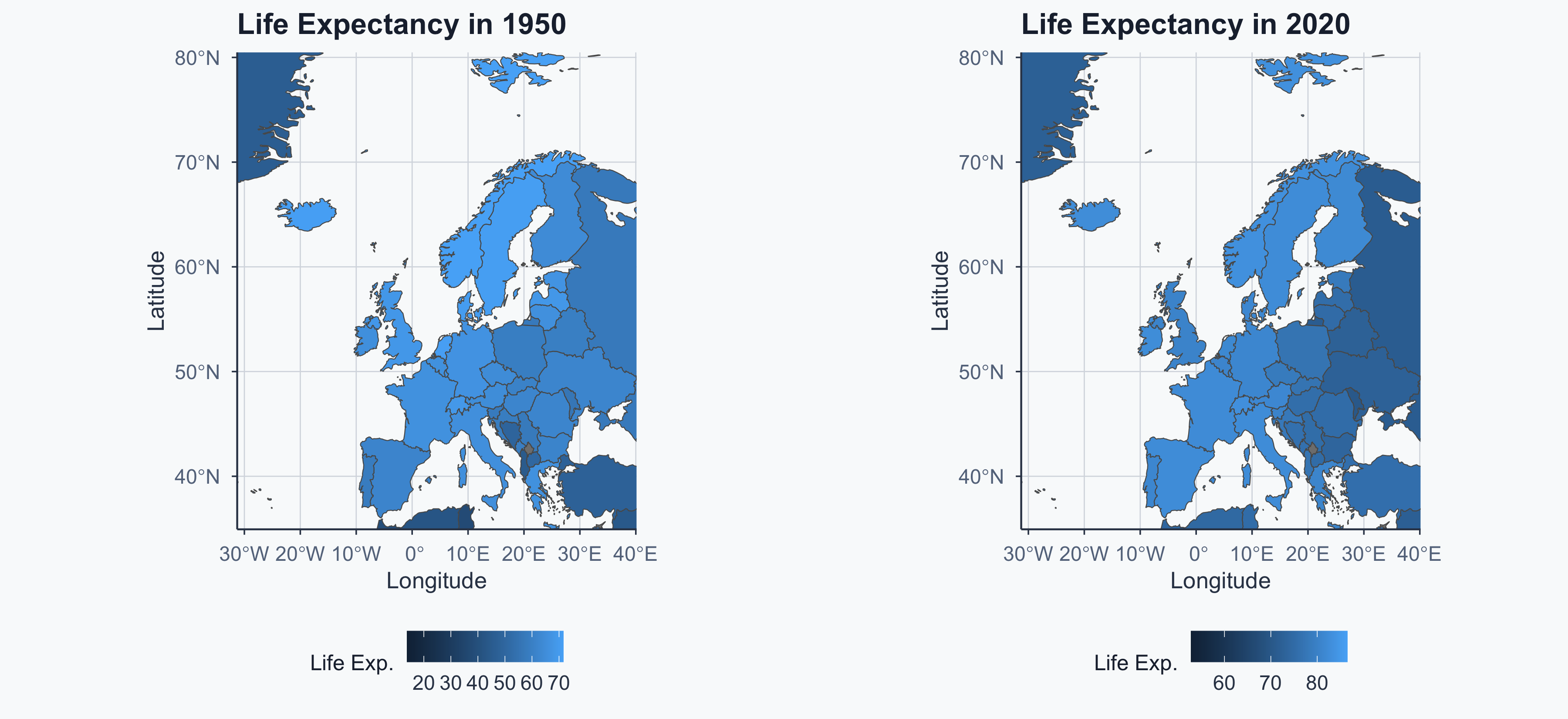
Hard to compare — the color scales differ between maps!
1950 vs 2020: Common Scale
Show code
figure2 <- ggplot() +
  geom_sf(data = world_1950, aes(fill = life_exp_mean)) +
  coord_sf(
    xlim = c(min_lon_x, max_lon_x),
    ylim = c(min_lat_y, max_lat_y),
    expand = FALSE
  ) +
  scale_fill_gradient(
    limits = c(vmin, vmax), name = "Life Expectancy"
  ) +
  labs(title = "1950", x = "Longitude", y = "Latitude") +
  theme_meridian()

figure3 <- ggplot() +
  geom_sf(data = world_2020, aes(fill = life_exp_mean)) +
  coord_sf(
    xlim = c(min_lon_x, max_lon_x),
    ylim = c(min_lat_y, max_lat_y),
    expand = FALSE
  ) +
  scale_fill_gradient(
    limits = c(vmin, vmax), name = "Life Expectancy"
  ) +
  labs(title = "2020", x = "Longitude", y = "Latitude") +
  theme_meridian()

ggarrange(figure2, figure3, ncol = 2, common.legend = TRUE)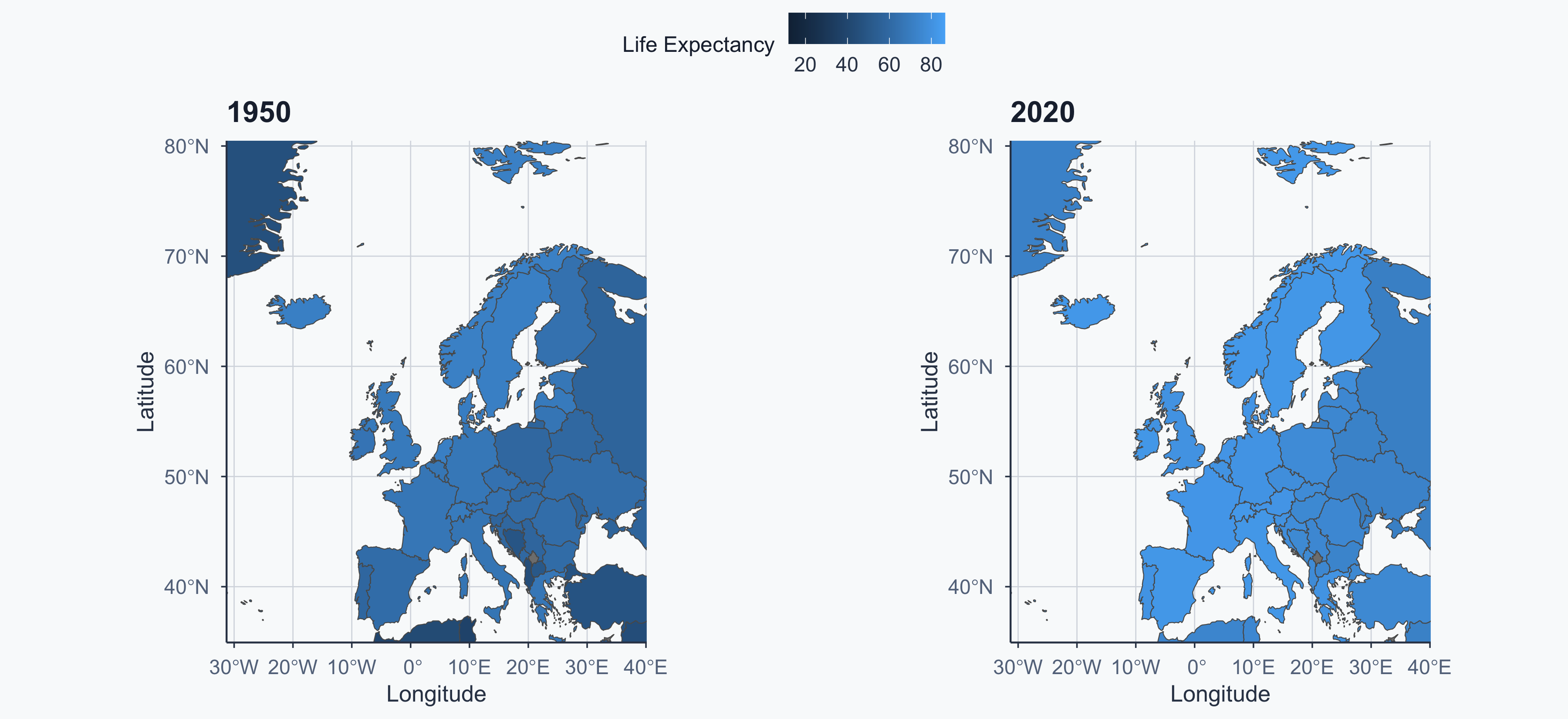
Map: Change in Life Expectancy
Show code
world_change <- left_join(
  world2, life_expectancy_1950_2020c,
  by = c("adm0_a3" = "Code")
)

ggplot() +
  geom_sf(data = world_change, aes(fill = differ)) +
  coord_sf(
    xlim = c(min_lon_x, max_lon_x),
    ylim = c(min_lat_y, max_lat_y),
    expand = FALSE
  ) +
  labs(
    title = "Life Expectancy Change: 2020 - 1950",
    x = "Longitude", y = "Latitude",
    fill = "Change",
    caption = "Source: Our World in Data"
  ) +
  theme_meridian()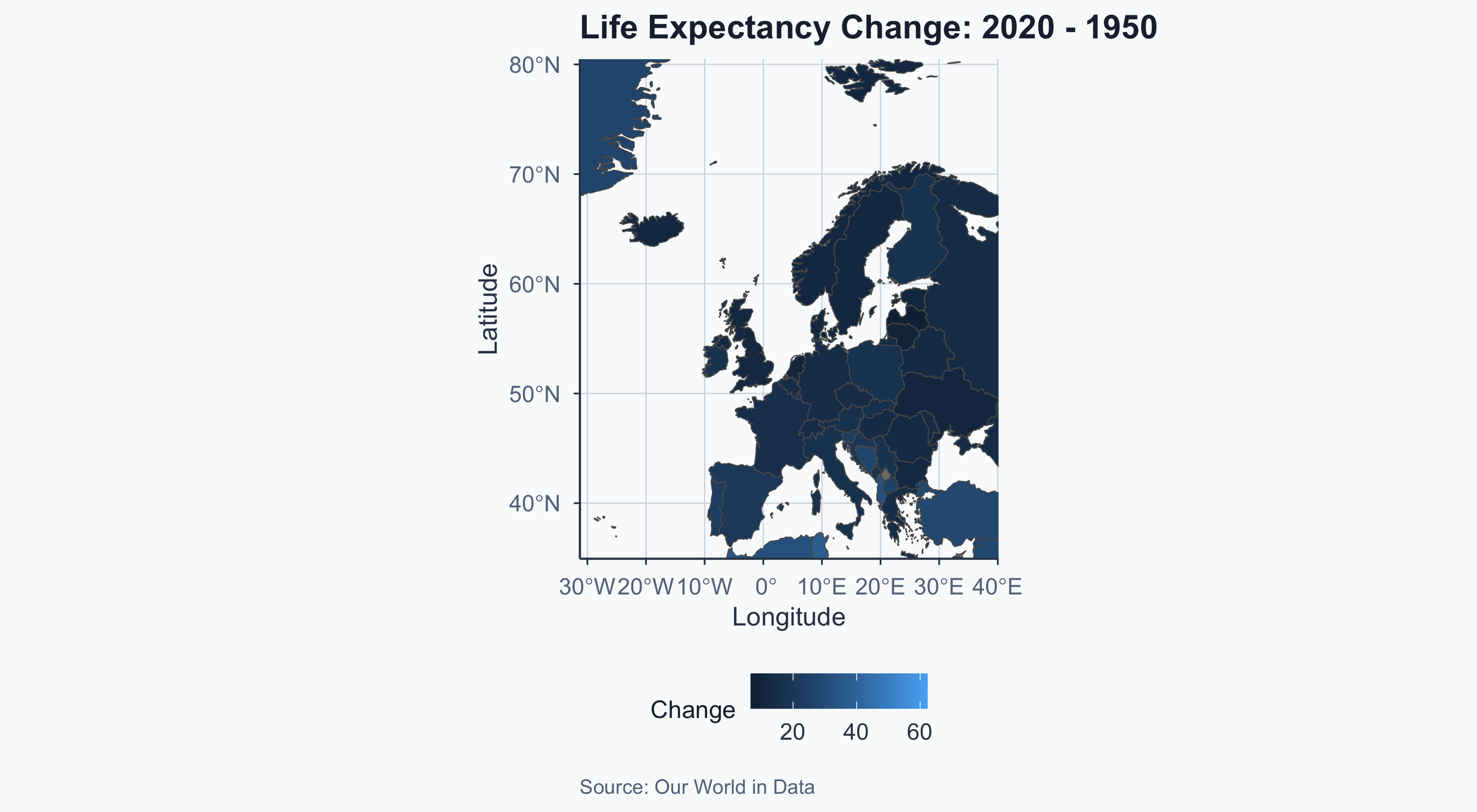
Scatterplot: Earliest Year (1960)
Show code
merged_earliest <- subset(merged_df2, Year == earliest_year)

cor_earliest <- round(
  cor(merged_earliest$life_exp_mean, merged_earliest$urb_mean), 2
)

ggplot(merged_earliest, aes(x = urb_mean, y = life_exp_mean)) +
  geom_point(alpha = 0.6, color = sage, size = 2) +
  geom_smooth(method = "lm", color = terracotta, se = FALSE) +
  coord_cartesian(xlim = x_lim, ylim = y_lim) +
  labs(
    title = paste0("Life Expectancy vs Urbanization (", earliest_year, ")"),
    subtitle = paste0("r = ", cor_earliest,
                      " · Each point = one country"),
    x = "Urban Population (%)",
    y = "Life Expectancy at Birth",
    caption = "Source: Our World in Data"
  ) +
  theme_meridian()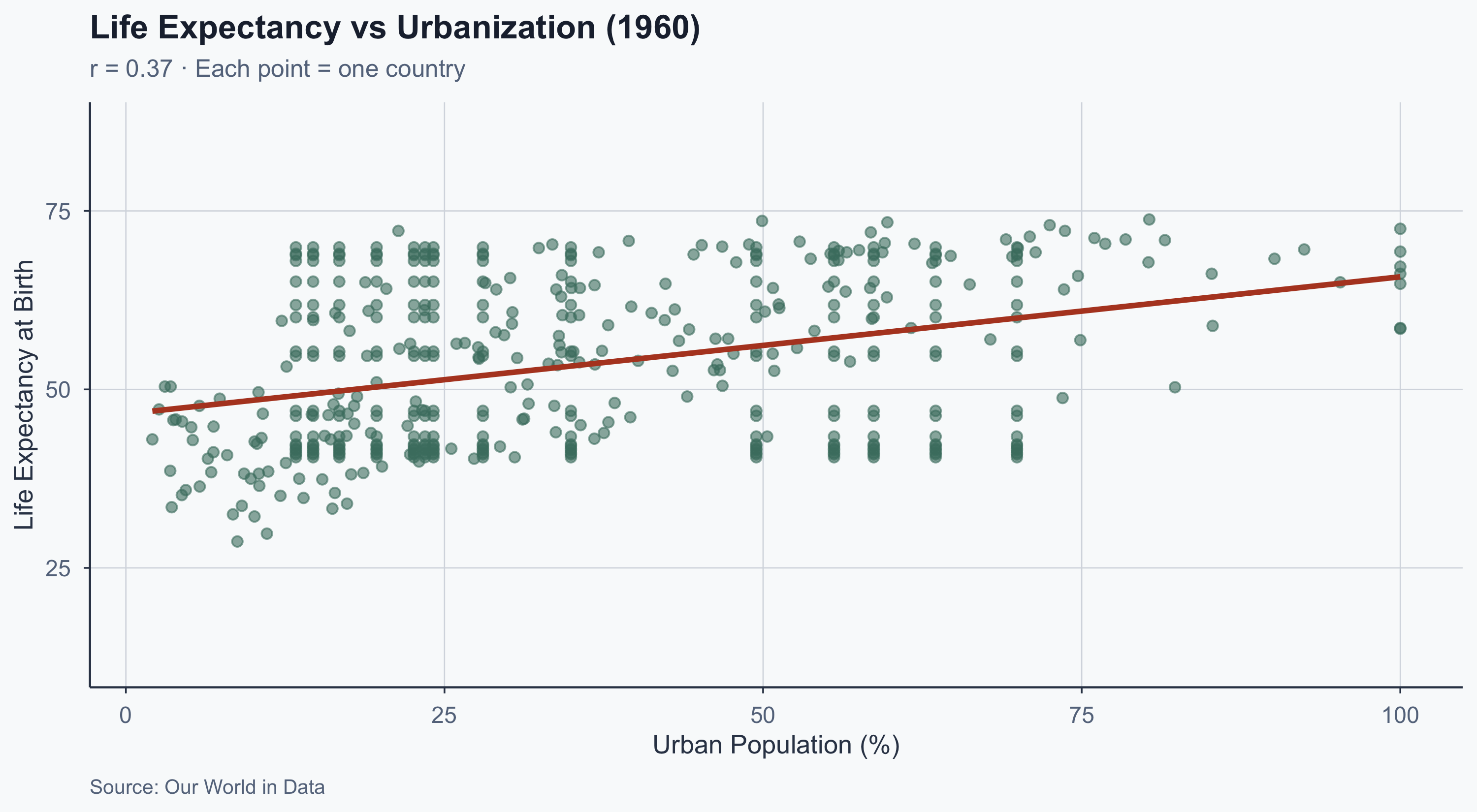
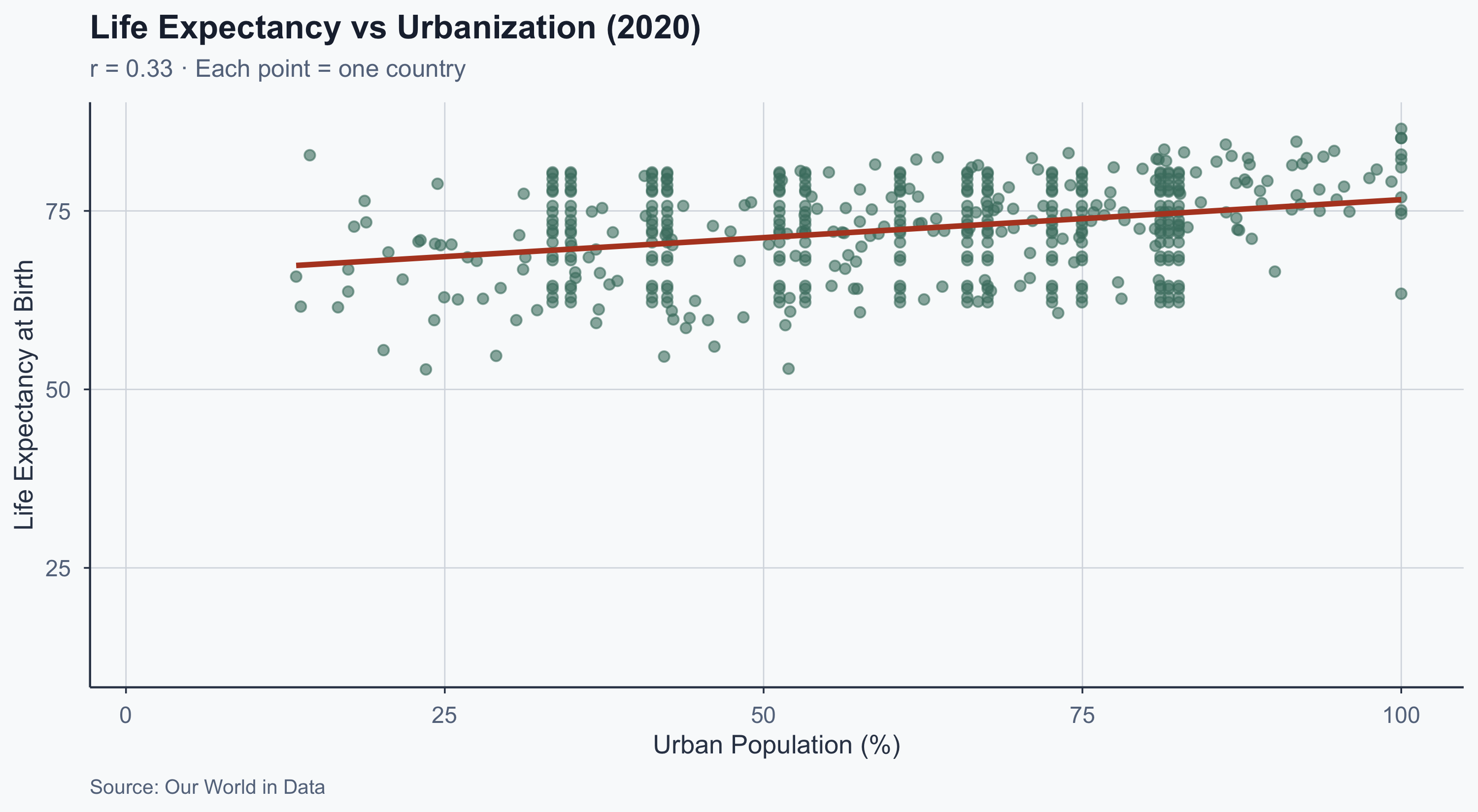
Scatterplot: Latest Year (2020)
Show code
merged_latest <- subset(merged_df2, Year == latest_year)

cor_latest <- round(
  cor(merged_latest$life_exp_mean, merged_latest$urb_mean), 2
)

ggplot(merged_latest, aes(x = urb_mean, y = life_exp_mean)) +
  geom_point(alpha = 0.6, color = sage, size = 2) +
  geom_smooth(method = "lm", color = terracotta, se = FALSE) +
  coord_cartesian(xlim = x_lim, ylim = y_lim) +
  labs(
    title = paste0("Life Expectancy vs Urbanization (", latest_year, ")"),
    subtitle = paste0("r = ", cor_latest,
                      " · Each point = one country"),
    x = "Urban Population (%)",
    y = "Life Expectancy at Birth",
    caption = "Source: Our World in Data"
  ) +
  theme_meridian()