Statistical Analysis

Lecture 6: Statistical Significance Testing and Z-Tests

Bogdan G. Popescu

John Cabot University

Outline

  • Review: sampling and probability distributions
  • Sampling distributions and the CLT
  • Statistical inference: samples vs populations
  • Seven steps of hypothesis testing (NHST)
  • One-sample and two-sample z-tests
  • Type I and Type II errors

Review

Previously

  • Researchers draw samples from populations
  • Multiple samples build a probability distribution
  • Sample statistics estimate population parameters

Sampling Illustration

Sampling from a population creates a distribution of sample means

EU Urbanization Distribution

Sampling Distributions

Sampling with Replacement

  • Select an item, record it, put it back
  • Repeat to create one random sample
  • Allows many samples from small groups
  • Simulates repeated sampling from population
  • Essential for estimating sampling distributions

Example: Sampling EU Countries

  • Consider: France, Germany, Italy, Spain, Netherlands
  • One sample: France, Germany, Germany, Spain, Italy
  • Germany appears twice (replacement allows this)
  • Repeat this process 1000+ times
  • Compute mean urbanization for each sample

50 Sample Means (EU)

1000 Sample Means (EU)

Central Limit Theorem

  • As sample count grows, distribution approaches normality
  • Holds regardless of population distribution shape
  • Larger samples produce narrower distributions
  • Enables hypothesis testing with z-scores

Why Sample?

  • Full population data: no sampling needed
  • Usually we lack access to entire population
  • Samples let us infer population characteristics
  • Goal: use sample to make population-level inferences

Statistical Inference

Key Concepts

  • Statistical inference: recovering population properties from samples
  • Population parameter: \(\theta\) (e.g., \(\mu\))
  • Sample statistic: \(\hat{\theta}\) (e.g., \(\bar{X}\))
  • \(\hat{\theta}\) has a sampling distribution
  • \(\bar{X}\) estimates \(\mu\)

Sample vs Population Mean

  • If \(\bar{X} \approx \mu\), sample is representative
  • We call \(\bar{X} = \mu\) the null hypothesis
  • Hypothesis testing evaluates this claim

The Z-Test

  • Tests whether a sample is typical of population
  • Appropriate when sample size \(n > 30\)
  • Assumes approximately normal distribution
  • Alternative for \(n < 30\): t-test

NHST: Seven Steps

Steps Overview

  1. Form comparison groups
  2. Define the null hypothesis (\(H_0\))
  3. Set significance level (\(\alpha\))
  4. Choose one-tailed or two-tailed test
  5. Find the critical value (\(Z_{crit}\))
  6. Calculate the test statistic (\(Z_{obs}\))
  7. Compare and decide

Running Example

  • EU researchers studied urbanization and life expectancy
  • Follow-up study examines Latin American countries
  • Question: Is Latin America typical of the world?

Step 1: Form Groups

Step 1: Form Groups

  • Z-test compares sample to population (or two samples)
  • Sample: Latin American countries
  • Population: all countries worldwide
  • Goal: determine if sample is representative
  • If typical: urbanization relates to life expectancy globally
  • If different: revisit the relationship

Step 2: Define H₀

Step 2: Define the Null Hypothesis

  • Null hypothesis: sample mean equals population mean
  • \(H_0: \bar{X} = \mu\)
  • Represents “no difference” or “no effect”

Step 3: Set Alpha

Step 3: Set Alpha (\(\alpha\))

  • \(\alpha\) = size of the rejection region
  • Ranges from 0 to 1
  • Convention: \(\alpha = 0.05\) (5% significance)

Alpha: Right Tail

Alpha: Left Tail

Alpha: Two Tails

Step 4: Choose Tails

One-Tailed Test

  • Entire rejection region in one tail
  • Tests if value is greater or less than reference
  • \(H_1: \bar{X} > \mu\) (right-tailed)
  • \(H_1: \bar{X} < \mu\) (left-tailed)

Two-Tailed Test

  • Rejection region split between both tails
  • Tests if value is different from reference
  • \(H_1: \bar{X} \neq \mu\)

Alternative Hypotheses Summary

Summary of alternative hypotheses
Test Type \(H_1\) Use When
Right-tailed \(\bar{X} > \mu\) Testing “greater than”
Left-tailed \(\bar{X} < \mu\) Testing “less than”
Two-tailed \(\bar{X} \neq \mu\) Testing “different from”

Step 5: Find the Critical Value

Step 5: Critical Value

  • Point where the rejection region starts
  • Beyond this value: rejection region
  • Determined by \(\alpha\) and test direction

Rejection Region: Right-Tailed

Rejection Region: Two-Tailed

Z-Table Reference

The critical value can be found in a standard normal (z) table.

  • Column A: z-score
  • Column B: area between mean and z
  • Column C: area in the tail beyond z

Urbanization: Latin America

Latin America vs World

Population Parameters

  • Population mean (\(\mu\)): 51.48
  • Population SD (\(\sigma\)): 24.14
  • Latam sample mean (\(\bar{X}\)): 59.02
  • Latam sample size (\(n\)): 23

Two-Tailed Z-Test Setup

Is the Latin American mean different from the world mean?

\[H_0: \bar{X}_{Latam} = \mu\]

\[H_1: \bar{X}_{Latam} \neq \mu\]

Z-Test: R Code

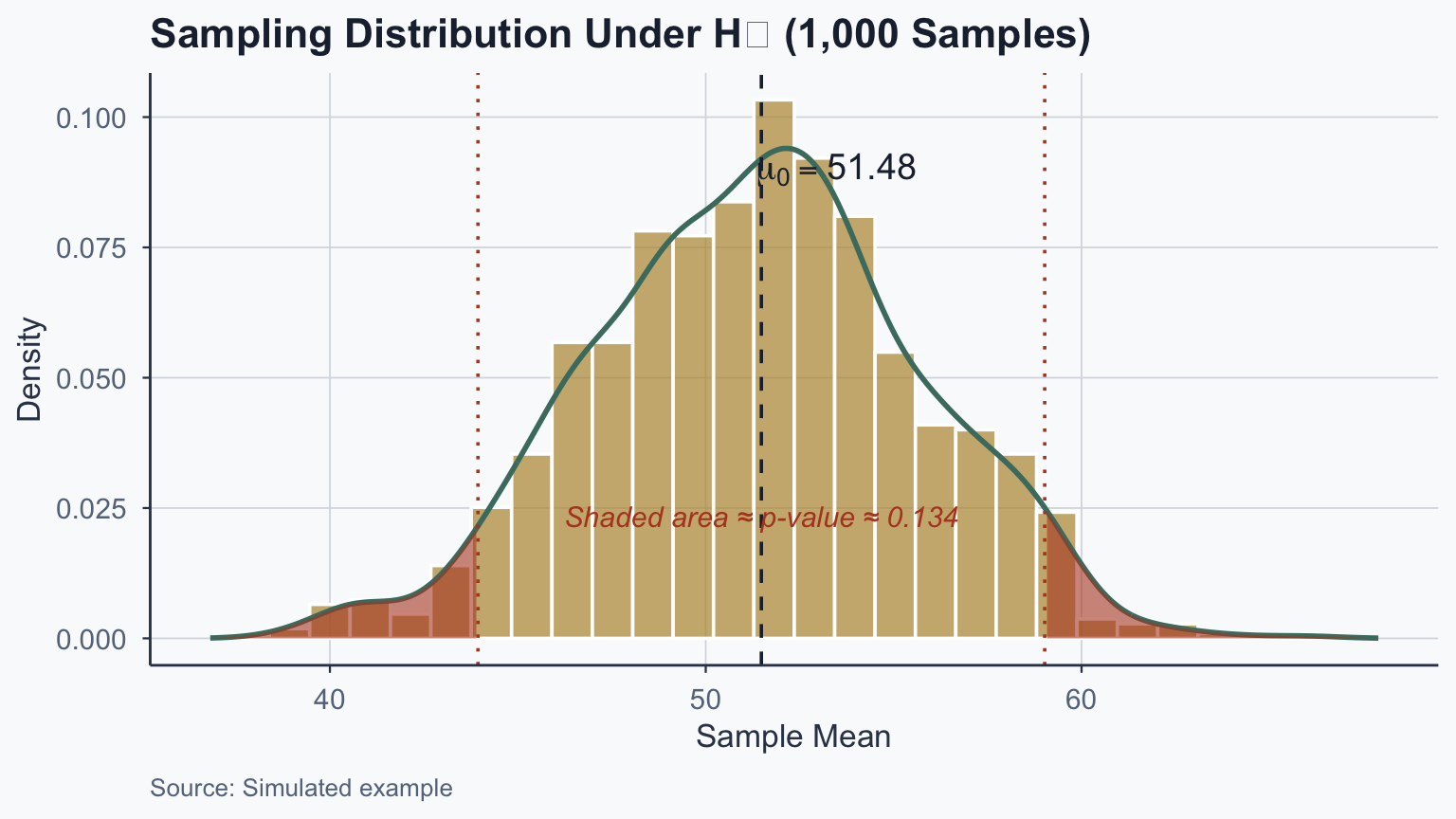
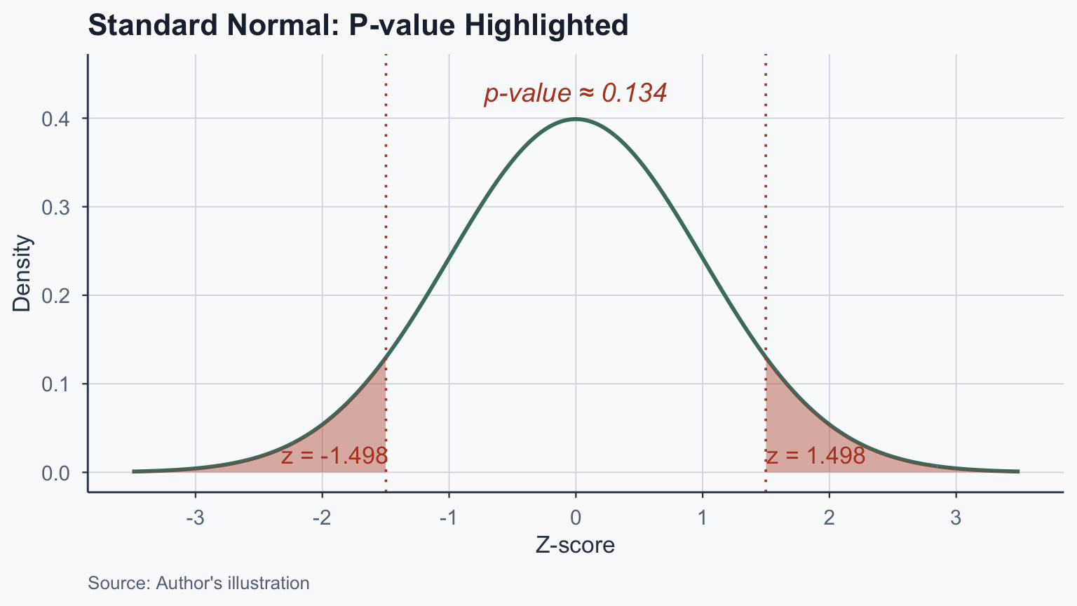
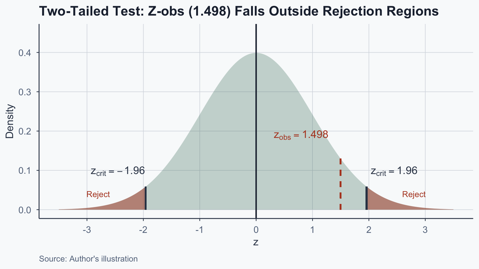
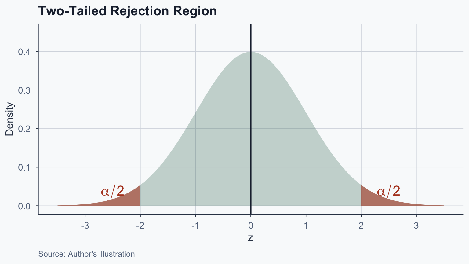
# One-sample z-test (manual computation)
z_obs_1 <- (latam_mean - pop_mean) / (pop_sd / sqrt(n_latam))
p_value_1 <- 2 * (1 - pnorm(abs(z_obs_1)))
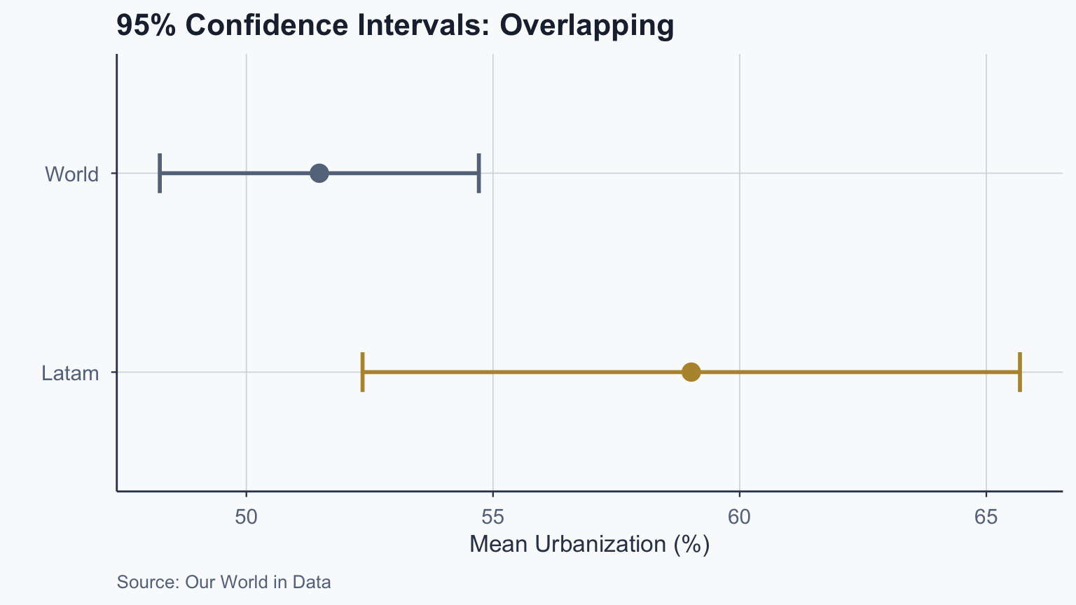
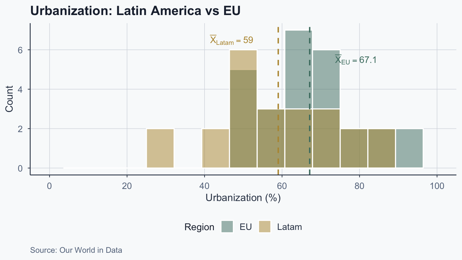
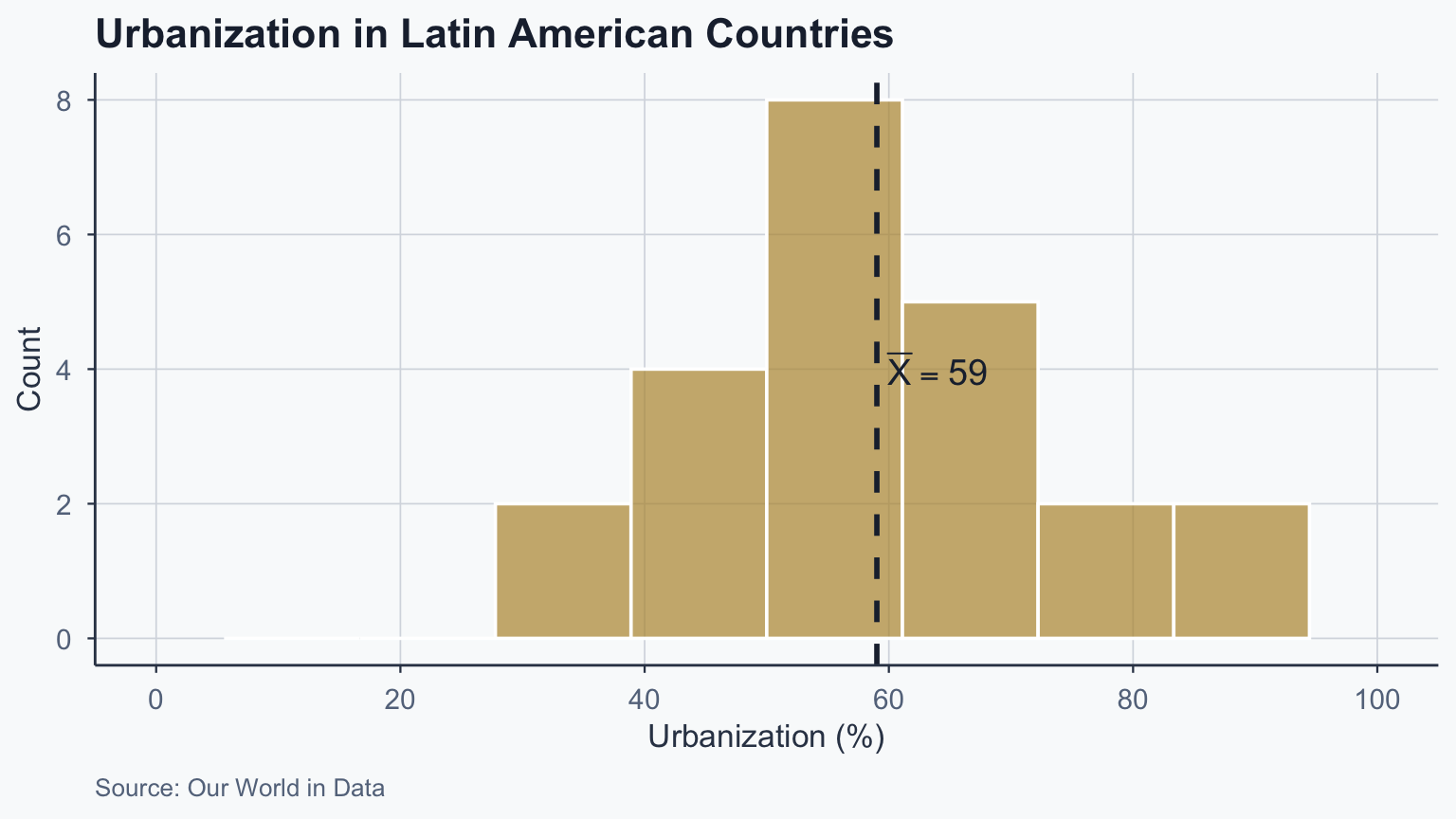
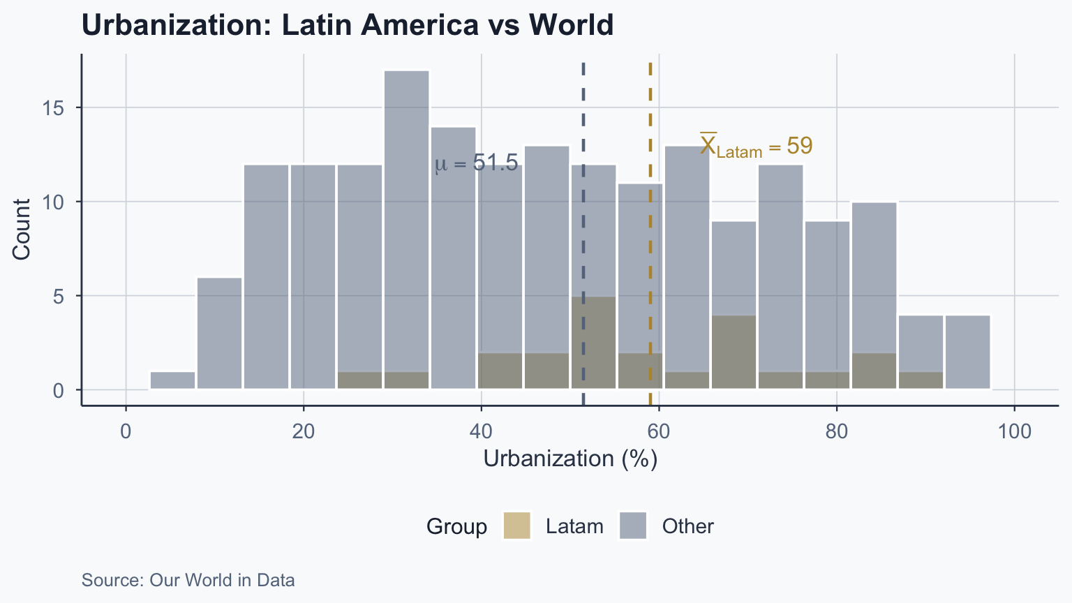
cat("z =", round(z_obs_1, 3), "\n")
z = 1.498 
cat("p-value =", round(p_value_1, 4), "\n")
p-value = 0.1341 
cat("Sample mean:", round(latam_mean, 2), "\n")
Sample mean: 59.02 
cat("Population mean:", round(pop_mean, 2))
Population mean: 51.48

Z-Test: Interpretation

  • \(z = 1.498\), \(p = 0.134\)
  • \(p\text{-value } (0.134) > \alpha \ (0.05)\)
  • Do not reject \(H_0\)
  • Insufficient evidence that Latam differs from world

Interpreting the P-value

What Is the P-value?

  • Probability of observing result this extreme under \(H_0\)
  • Assumes the null hypothesis is true
  • Small p-value: result is unlikely under \(H_0\)
  • Large p-value: result is consistent with \(H_0\)

Simulated Sampling Distribution

P-value on the Standard Normal

Confidence Intervals: Latam vs World

P-value Decision Rule

  • If \(p < 0.05\): reject \(H_0\)
  • If \(p > 0.05\): do not reject \(H_0\)
  • Our result: \(p = 0.134 > 0.05\)
  • Overlapping CIs confirm this conclusion

Step 6: Calculate Z_obs

Z-obs Formula

\[Z_{obs} = \frac{\bar{X} - \mu}{\frac{\sigma}{\sqrt{n}}}\]

Plugging in values:

\[Z_{obs} = \frac{59.02 - 51.48}{\frac{24.14}{\sqrt{23}}} = 1.498\]

Z-obs Matches R Output

z_obs_manual <- (latam_mean - pop_mean) / (pop_sd / sqrt(n_latam))
cat("Z_obs (manual):", round(z_obs_manual, 3))
Z_obs (manual): 1.498

Step 7: Compare & Decide

Comparing Z-obs to Z-crit

  • \(Z_{obs} = 1.498\)
  • \(Z_{crit}\) for \(\alpha = 0.05\) (two-tailed): \(\pm 1.96\)
  • \(|1.498| < 1.96\): not in rejection region
  • Cannot reject \(H_0: \bar{X}_{Latam} = \mu\)

Visual: Z-obs vs Z-crit

Conclusion for One-Sample Test

  • \(|Z_{obs}| = 1.498 < Z_{crit} = 1.96\)
  • Fail to reject \(H_0\)
  • Latin American urbanization not significantly different
  • Consistent with world mean

Two-Sample Z-Test

Latin America vs EU

Summary Statistics

Urbanization summary statistics by region
Parameter Latam EU World
Mean 59 67.1 51.5
SD 16.3 13.1 24.1
n 23 27 214

Two-Sample Z-Test: Setup

Steps 1–4 applied to two groups:

  • Step 1: Groups = Latam vs EU
  • Step 2: \(H_0: \bar{X}_{Latam} - \bar{X}_{EU} = 0\)
  • Step 3: \(\alpha = 0.05\)
  • Step 4: Two-tailed (\(\neq\))

\[H_1: \bar{X}_{Latam} - \bar{X}_{EU} \neq 0\]

Two-Sample Z-Test: Results

# Two-sample z-test (manual)
z_obs_2 <- (latam_mean - eu_mean) /
  sqrt(latam_sd^2 / n_latam + eu_sd^2 / n_eu)
p_value_2 <- 2 * (1 - pnorm(abs(z_obs_2)))

cat("z =", round(z_obs_2, 4), "\n")
z = -1.9176 
cat("p-value =", round(p_value_2, 4))
p-value = 0.0552

Two-Sample: Steps 5–7

  • Step 5: \(Z_{crit} = \pm 1.96\) (two-tailed, \(\alpha = 0.05\))
  • Step 6: \(z = -1.918\), \(p = 0.0552\)
  • Step 7: \(p (0.055) > 0.05\)do not reject \(H_0\)
  • Difference in urbanization not statistically significant

Confidence Intervals: Latam vs EU

One-Tailed Tests

One-Tailed: Greater Than

Step 4 changes to one-tailed; Step 5: \(Z_{crit} = 1.64\)

# H0: Latam mean is NOT greater than population mean
# H1: Latam mean IS greater than population mean
z_obs_gt <- (latam_mean - pop_mean) / (pop_sd / sqrt(n_latam))
p_gt     <- 1 - pnorm(z_obs_gt)

cat("z =", round(z_obs_gt, 3), "\n")
z = 1.498 
cat("p-value =", round(p_gt, 4))
p-value = 0.0671
  • Step 7: \(p > 0.05\)do not reject \(H_0\)

One-Tailed: Less Than

Step 4 changes direction; Step 5: \(Z_{crit} = -1.64\)

# H0: Latam mean is NOT less than population mean
# H1: Latam mean IS less than population mean
p_lt <- pnorm(z_obs_gt)

cat("z =", round(z_obs_gt, 3), "\n")
z = 1.498 
cat("p-value =", round(p_lt, 4))
p-value = 0.9329
  • Step 7: \(p > 0.05\)do not reject \(H_0\)

One-Tailed vs Two-Tailed Recap

  • One-tailed: tests one direction (greater or less)
  • Two-tailed: tests both directions (different from)
  • Same z-statistic, different p-value calculation
  • Two-tailed p-value = 2 \(\times\) one-tailed p-value

Type I & Type II Errors

Error Types

  • Type I error: reject a true \(H_0\) (false positive)
  • Type II error: retain a false \(H_0\) (false negative)

Error Summary

Decision outcomes in hypothesis testing
\(H_0\) True \(H_0\) False
Reject \(H_0\) Type I Error (\(\alpha\)) Correct
Retain \(H_0\) Correct Type II Error (\(\beta\))

Applied Example: Latam Urbanization

Our test: \(H_0\): Latam urbanization = world mean

  • Type I error here: conclude Latam differs from the world when it actually does not
    • Could lead to misallocated urban development funds
  • Type II error here: conclude Latam matches the world when it actually differs
    • Could miss real urbanization disparities
  • We set \(\alpha = 0.05\) — accepting a 5% risk of Type I error

Real-World Applications

Where NHST Applies

  • Medical trials: new drug vs placebo effectiveness
  • Education: new teaching method vs traditional scores
  • Climate: recent temperatures vs historical averages
  • Policy: program impact vs no-intervention baseline

Conclusion

What You Can Now Do

  • Formulate null and alternative hypotheses for real problems
  • Choose between one-tailed and two-tailed z-tests
  • Compute and interpret z-scores and p-values
  • Use confidence intervals to visualize group differences
  • Recognize Type I / Type II error trade-offs

Why This Matters

  • Every empirical claim in social science rests on NHST
  • “Is this pattern real or just noise?” is now answerable
  • Next step: t-tests for small samples (\(n < 30\))

Practice

Practice 1

Interpret the following two-sample z-test output:

Two-sample z-Test
data: final_latam$life_expectancy and final_eu$life_expectancy
z = -2.0453, p-value = 0.0409
alternative hypothesis: true difference in means is not equal to 0
95% confidence interval: -6.42  -0.18
sample estimates:
mean of x  mean of y
    73.84      77.14

Practice 2

Interpret the following one-sample z-test output:

One-sample z-Test
data: na.omit(final_eu$life_expectancy)
z = 2.305, p-value = 0.0212
alternative hypothesis: true mean is not equal to 75
95% confidence interval: 75.82  80.46
sample estimates:
mean of x
    78.14

Practice 3

Interpret the following one-sample z-test output:

One-sample z-Test
data: na.omit(final_latam$life_expectancy)
z = 1.765, p-value = 0.0776
alternative hypothesis: true mean is not equal to 75
95% confidence interval: 72.34  78.89
sample estimates:
mean of x
    76.12

Practice 4

Interpret the following two-sample z-test output:

Two-sample z-Test
data: final_latam$life_expectancy and final_eu$life_expectancy
z = 1.5624, p-value = 0.1181
alternative hypothesis: true difference in means is not equal to 0
95% confidence interval: -0.87132  3.12345
sample estimates:
mean of x  mean of y
    74.56      72.89