Statistical Analysis

Lecture 5: Probability II

Bogdan G. Popescu

bogdan.popescu@johncabot.edu

John Cabot University

Discrete vs. Continuous Variables

Discrete Variables

• Finite, countable, non-negative integers
• Examples: number of children, dice rolls

Continuous Variables

• Infinitely many values within a range
• Often carry decimal points
• Examples: height, weight, temperature

Histograms

What Is a Histogram?

• Shows values and how often each appears
• Describes the distribution of a variable
• Works for both discrete and continuous data
• A complete description of the sample

Life Expectancy: Histogram

Figure 1: Distribution of average life expectancy by country

Probability Mass Functions

What Is a PMF?

• Shows the probability of each discrete value
• Divide each frequency by total observations \(n\)
• All probabilities must sum to 1
• Describes the probability distribution

PMF Example: Class Grades

Grades of 10 students: 30, 30, 30, 60, 60, 80, 80, 80, 90, 100

Grade (\(x\))	30	60	80	90	100
Frequency	3	2	3	1	1
\(\mathbb{P}(X=x)\)	0.3	0.2	0.3	0.1	0.1

\(\mathbb{P}(X=30) = 0.3\): 30% chance of drawing grade 30.

PMF: Formal Definition

\[ \begin{aligned} f(x) &= \mathbb{P}(X=x) \quad \text{Each value has a probability}\\[0.3cm] f(x) &\geq 0 \quad \text{Probabilities cannot be negative}\\[0.3cm] \sum_{x} f(x) &= 1 \quad \text{All probabilities sum to 1} \end{aligned} \]

• PMF can be a formula, table, or figure
• Defined for every \(x\) in the support of \(X\)

PMF Example: Fair Coin Toss

Define \(X = 0\) (tails) and \(X = 1\) (heads).

\[ f(0) = \mathbb{P}(X = 0) = \tfrac{1}{2}, \quad f(1) = \mathbb{P}(X = 1) = \tfrac{1}{2} \]

\(x\)	0	1
\(\mathbb{P}(X=x)\)	0.5	0.5

PMF Example: Unfair Coin Toss

Define \(X = 0\) (tails) and \(X = 1\) (heads).

\[ f(0) = \mathbb{P}(X = 0) = \tfrac{1}{10}, \quad f(1) = \mathbb{P}(X = 1) = \tfrac{9}{10} \]

\(x\)	0	1
\(\mathbb{P}(X=x)\)	0.1	0.9

The Bernoulli Distribution

• Models experiments with exactly two outcomes
• Examples: coin toss, pass/fail, yes/no

\[ f(1) = \mathbb{P}(X=1) = p, \quad f(0) = \mathbb{P}(X=0) = 1-p \]

• \(p = 0.5\): fair coin (equally likely)
• \(p \neq 0.5\): biased coin
• Simplest PMF; building block for other models

PMF: General Definition

Variable \(X\) takes integer values from 1 to \(k\):

\[ \mathbb{P}(X = x) = p_x, \quad x = 1, 2, \dots, k \]

where \(p_x \geq 0\) and \(p_1 + p_2 + \dots + p_k = 1\).

Example: A 3-sided die —

\[ \mathbb{P}(X=1) = p_1, \quad \mathbb{P}(X=2) = p_2, \quad \mathbb{P}(X=3) = p_3 \]

Life Expectancy: PMF

Figure 2: PMF of average life expectancy by country

Histogram vs. PMF

Figure 3: Histogram shows raw frequencies

Figure 4: PMF shows probabilities

Limits of PMFs

• Work well when number of values is small
• As values increase, individual probabilities shrink
• Random noise becomes more apparent
• Solution: bin data into non-overlapping intervals
• Bin size is tricky: too large smooths signal

Binning in Action

Figure 5: Raw PMF: noisy, one bar per year

Figure 6: Binned PMF: smoother, 5-year intervals

Binning smooths out noise — but what happens as bins get infinitely narrow? We get a PDF.

Probability Density Functions

From Discrete to Continuous

Discrete: PMF gives \(\mathbb{P}(X = x)\) for each value.

Continuous: there are infinitely many possible values.

• What is the probability someone is exactly 170.000… cm tall?
• Among infinite possible heights, any single value has probability zero
• \(\mathbb{P}(X = x) = 0\) for any exact value \(x\)

From Discrete to Continuous (cont.)

So if \(\mathbb{P}(X = x) = 0\), how do we talk about probability?

We ask about ranges instead:

• \(\mathbb{P}(169 \leq X \leq 171)\) — perfectly well-defined
• \(\mathbb{P}(X \leq 175)\) — this is the CDF
• The tool that computes these range probabilities is the PDF

What Is a PDF?

\[ \mathbb{P}(a \leq X \leq b) = \int_a^b f(x)\,dx \]

• \(f(x)\) is a density, not a probability
• Probabilities come from areas under the curve
• Taller curve at \(x\) means values near \(x\) more likely

Intuition: Histogram to PDF

A PDF is a smoothed-out histogram as bins get finer.

Figure 7: 5 bins: coarse approximation

Figure 8: 100 bins: approaches the PDF

Properties of a PDF

1. Non-negative: \(f(x) \geq 0\) for all \(x\)
2. Total area equals 1: \(\int_{-\infty}^{\infty} f(x)\, dx = 1\)
3. Probability of a range: \(\mathbb{P}(a \leq X \leq b) = \int_{a}^{b} f(x)\, dx\)

\(f(x)\) is not a probability — it gives relative likelihood near \(x\).

PDF: Total Area Equals 1

Figure 9: Total area under the PDF curve equals 1

PDF: Probability of a Range

For a standard normal \(N(0,1)\):

\[\mathbb{P}(-1 \leq X \leq 1) = \int_{-1}^{1} f(x)\, dx\]

• No closed-form solution; use R: pnorm(1) - pnorm(-1)
• Result: \(\approx 0.683\) — about 68.3% within 1 SD

PDF: Probability of a Range (Visual)

Figure 10: Shaded area gives interval probability

Normal Distribution

What Is the Normal Distribution?

Also called the Gaussian or bell curve.

• Symmetric about the mean
• Mean = Median = Mode at the center
• Bell-shaped: data concentrated around mean
• Spread determined by standard deviation

Normal Distribution: Formula

\[ f(x) = \frac{1}{\sigma \sqrt{2\pi}} \exp\!\left(-\frac{(x-\mu)^2}{2\sigma^2}\right) \]

• Two parameters: \(\mu\) (mean) and \(\sigma\) (std. dev.)
• \(\mu\) controls location (center of curve)
• \(\sigma\) controls spread (width of curve)
• \(\sigma^2\) is the variance

Effect of the Mean (\(\mu\))

Figure 11: Changing the mean shifts the curve horizontally

Mean and Standard Deviation Annotated

Figure 12: Mean and one standard deviation boundaries

Effect of Standard Deviation (\(\sigma\))

Figure 13: Larger sigma produces wider, flatter curves

The 68-95-99.7 Rule

For any normal distribution:

Range	Probability
\(\mu \pm 1\sigma\)	68.3%
\(\mu \pm 2\sigma\)	95.4%
\(\mu \pm 3\sigma\)	99.7%

This is the empirical rule — the single most useful fact about normal distributions.

The 68-95-99.7 Rule (Visual)

Figure 14: The empirical rule for the standard normal

Standard Normal Distribution

The standard normal has \(\mu = 0\) and \(\sigma = 1\):

\[N(0, 1)\]

• Any normal can be standardized to \(N(0,1)\)
• Reference distribution in statistics
• Foundation for hypothesis testing

Cumulative Distribution Functions

What Are Percentiles?

• Standardized tests report a percentile rank
• Fraction of scores at or below yours
• 90th percentile = scored \(\geq\) 90% of takers

Formula:

\[P = \frac{\text{No. values} \leq X}{\text{Total no. of values}} \times 100\]

Percentile Example

Scores: 55, 66, 77, 88, 99. You scored 88.

\[P = \frac{4}{5} \times 100 = 80\]

Four values (55, 66, 77, 88) are \(\leq\) 88 \(\Rightarrow\) percentile rank = 80.

What if you scored 77?

\[P = \frac{3}{5} \times 100 = 60\]

What Is a CDF?

• Maps values to their percentile rank (as probability)
• Gives \(\mathbb{P}(X \leq x)\) for any value \(x\)
• Works for both discrete and continuous variables
• Always increases from 0 to 1

CDF: How It Works

For any value \(x\), the CDF counts:

\[F(x) = \frac{\text{No. values} \leq x}{\text{Total no. of values}}\]

• Same idea as the percentile formula, but expressed as a probability \([0, 1]\)
• For continuous distributions, R computes this with pnorm(x, mean, sd)

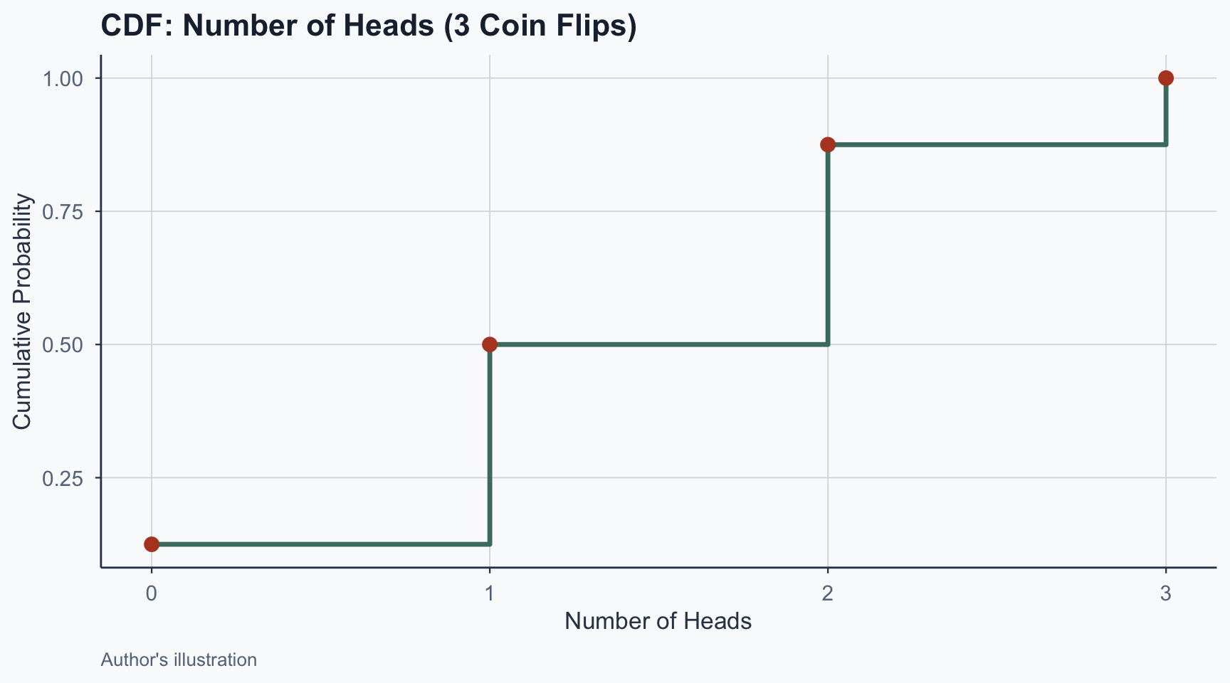
CDF Example: Three Coin Flips

Flip a fair coin 3 times. Total outcomes: \(2^3 = 8\).

Heads (\(k\))	0	1	2	3
Probability	1/8	3/8	3/8	1/8
Cumul. Prob.	0.125	0.500	0.875	1.000

Each probability: \(P(X=k) = \binom{3}{k}\left(\frac{1}{2}\right)^3\)

CDF: Coin Flips Plot

Figure 15: CDF for number of heads in 3 coin flips

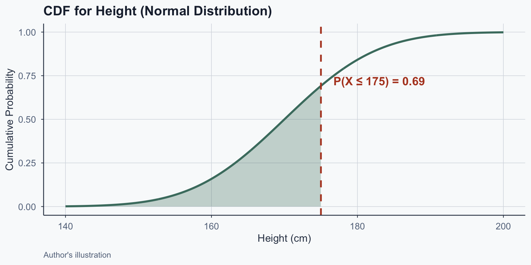
CDF: Continuous Example (Height)

Heights modeled as \(N(\mu = 170,\; \sigma = 10)\) cm.

Figure 16: CDF for height: P(X <= 175) = 0.69

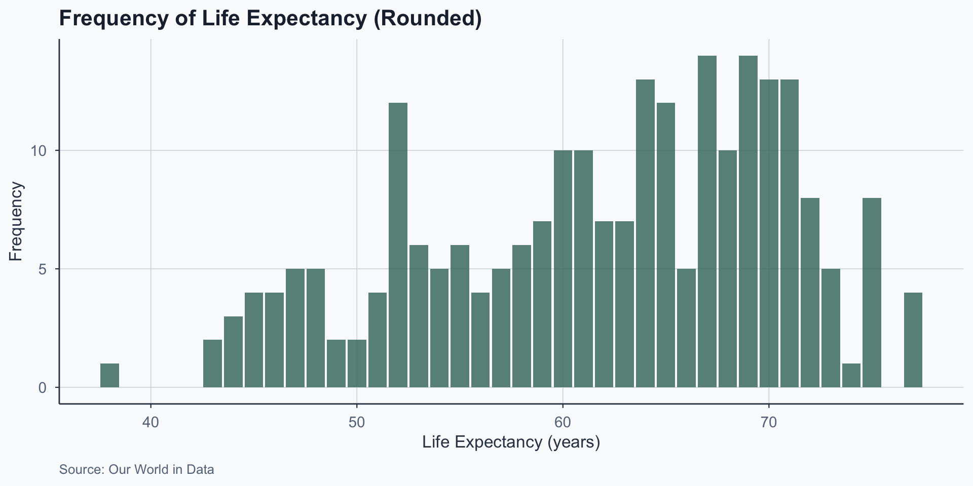
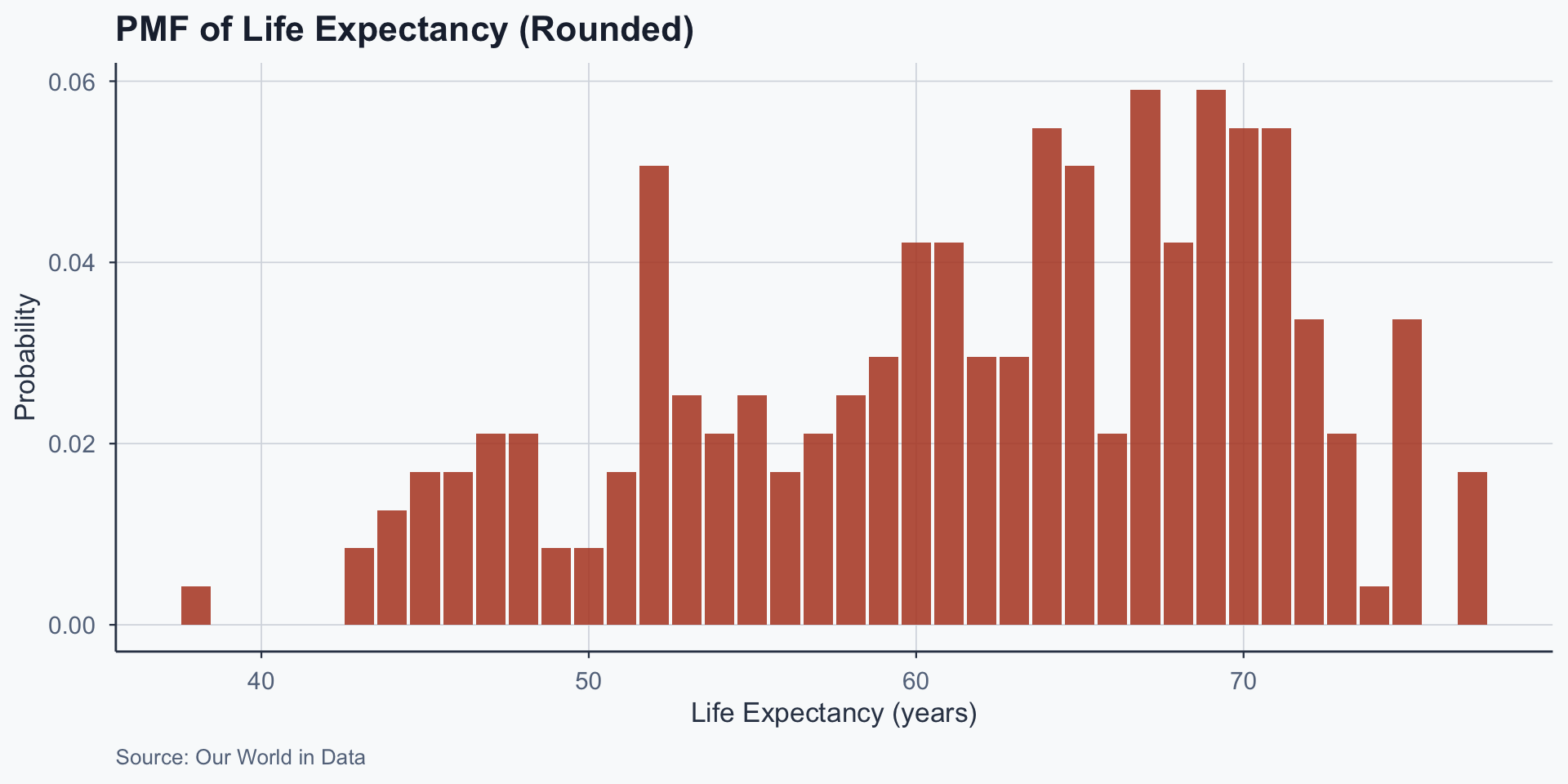
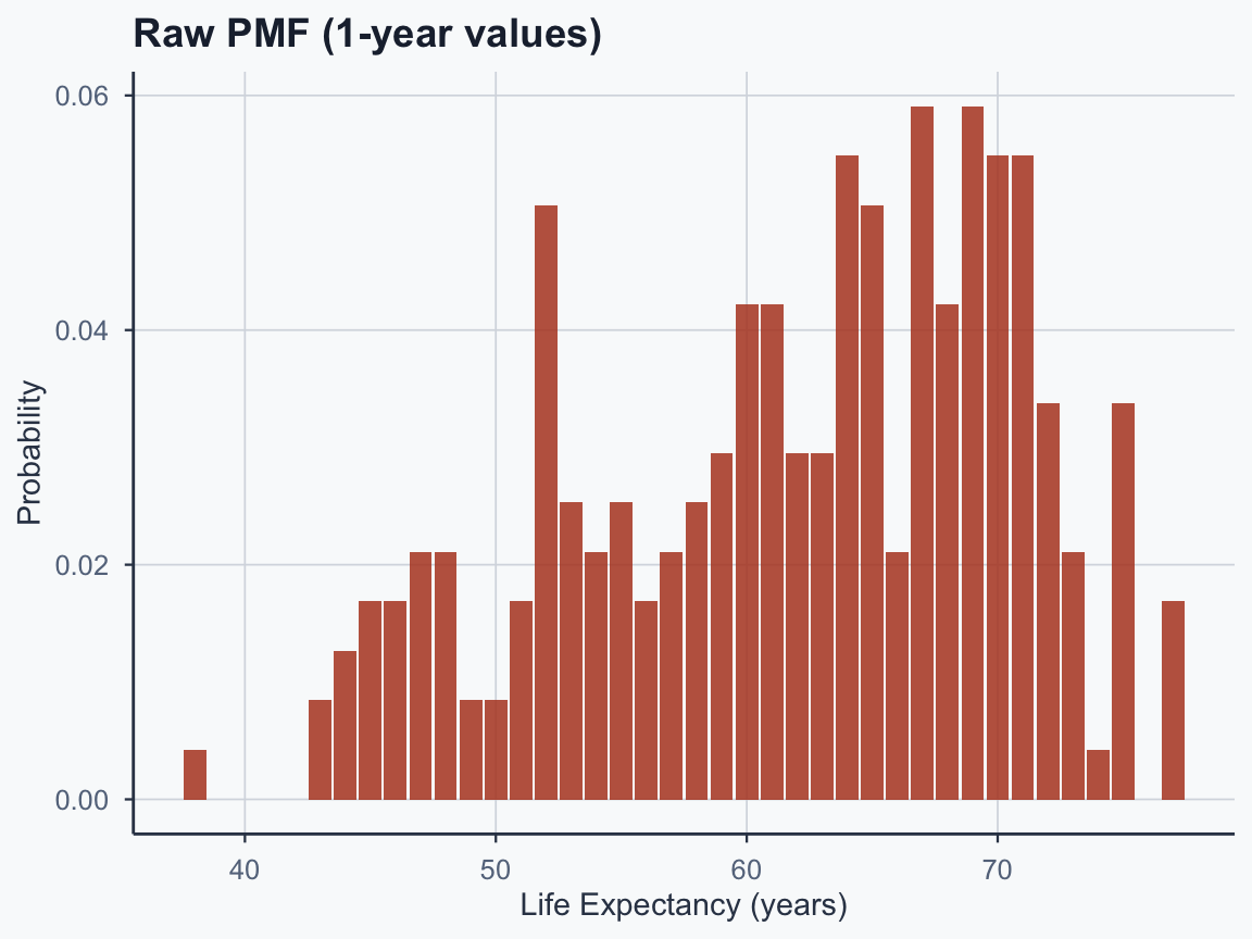
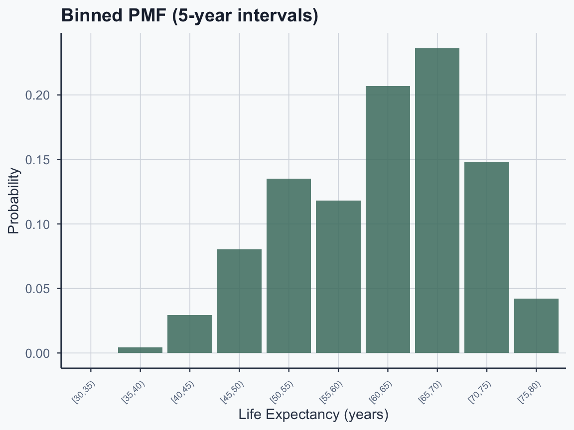
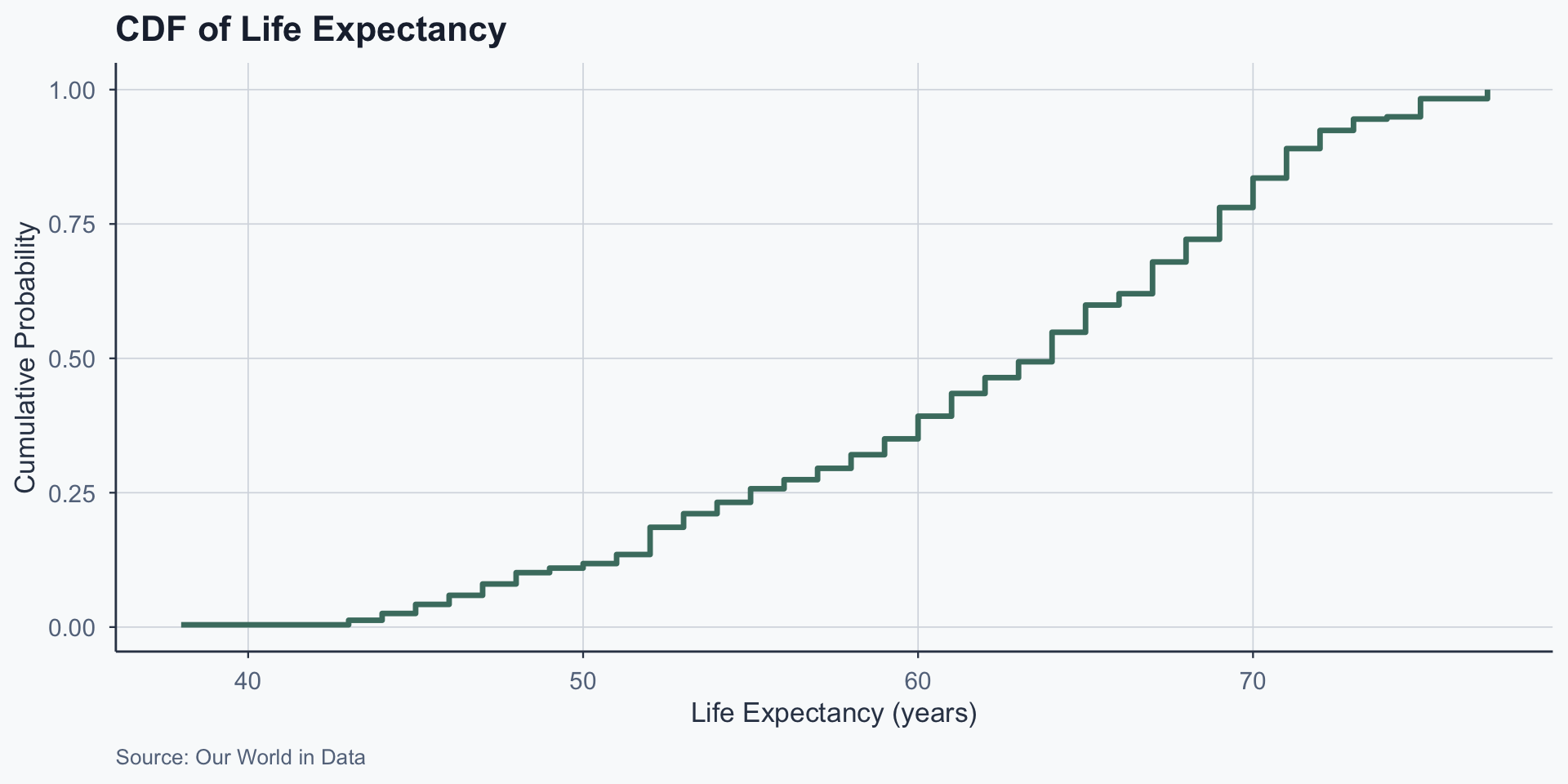
Life Expectancy: CDF

Figure 17: CDF of average life expectancy by country

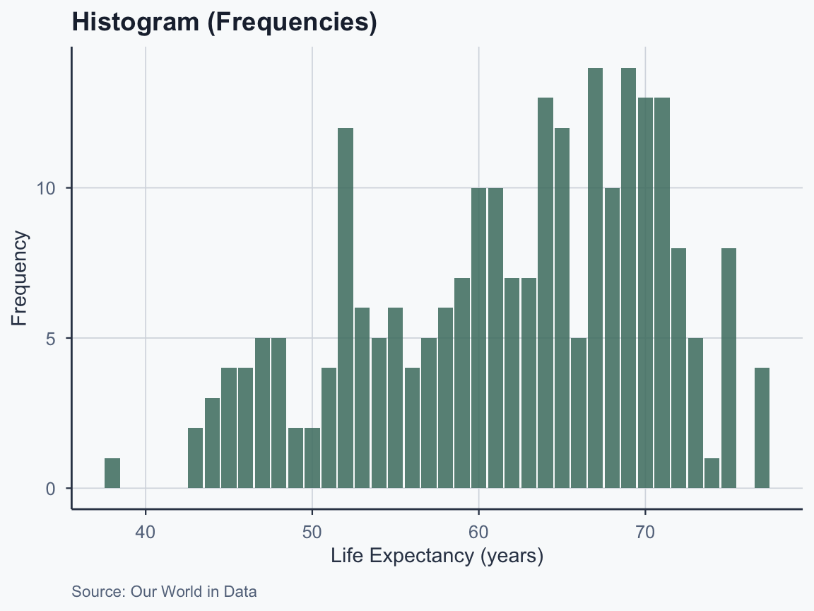
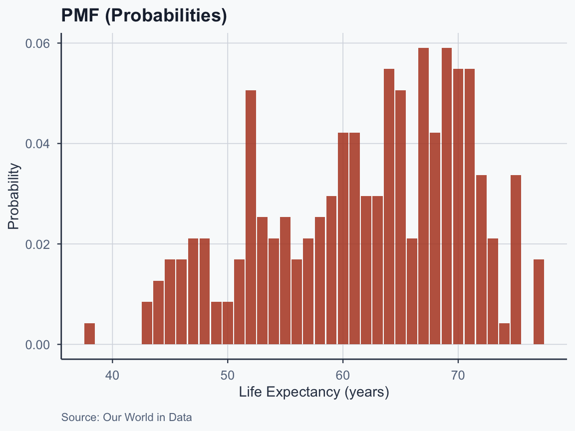
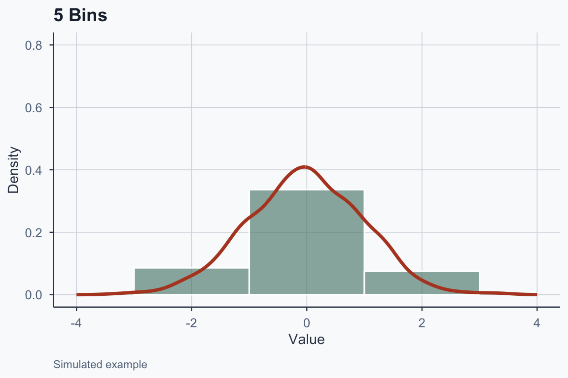
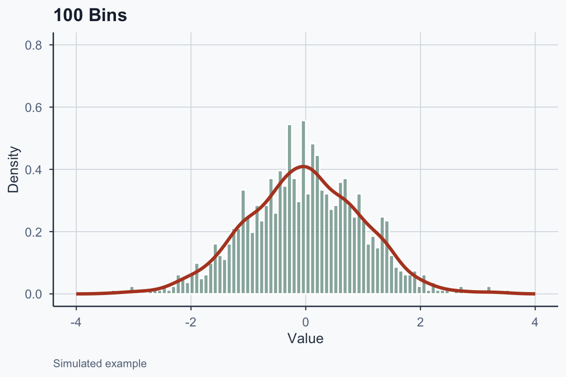
PMF vs. PDF vs. CDF

%%{init:{'flowchart':{'useMaxWidth':true,'nodeSpacing':60,'rankSpacing':60},'themeVariables':{'fontSize':'22px'}}}%%
flowchart LR
  A["Raw Data"] --> B["Histogram<br/>(Frequencies)"]
  B --> C["PMF<br/>(Discrete Prob.)"]
  B --> D["PDF<br/>(Continuous<br/>Density)"]
  C --> E["CDF<br/>(Cumulative<br/>Prob.)"]
  D --> E

Function	Variable Type	Gives
PMF	Discrete	\(\mathbb{P}(X = x)\)
PDF	Continuous	Density at \(x\)
CDF	Both	\(\mathbb{P}(X \leq x)\)

Conclusion

What Can You Do Now?

• Quantify uncertainty: given a distribution, compute the probability of any range of outcomes
• Compare: the CDF lets you answer “what fraction falls below this threshold?” for any dataset
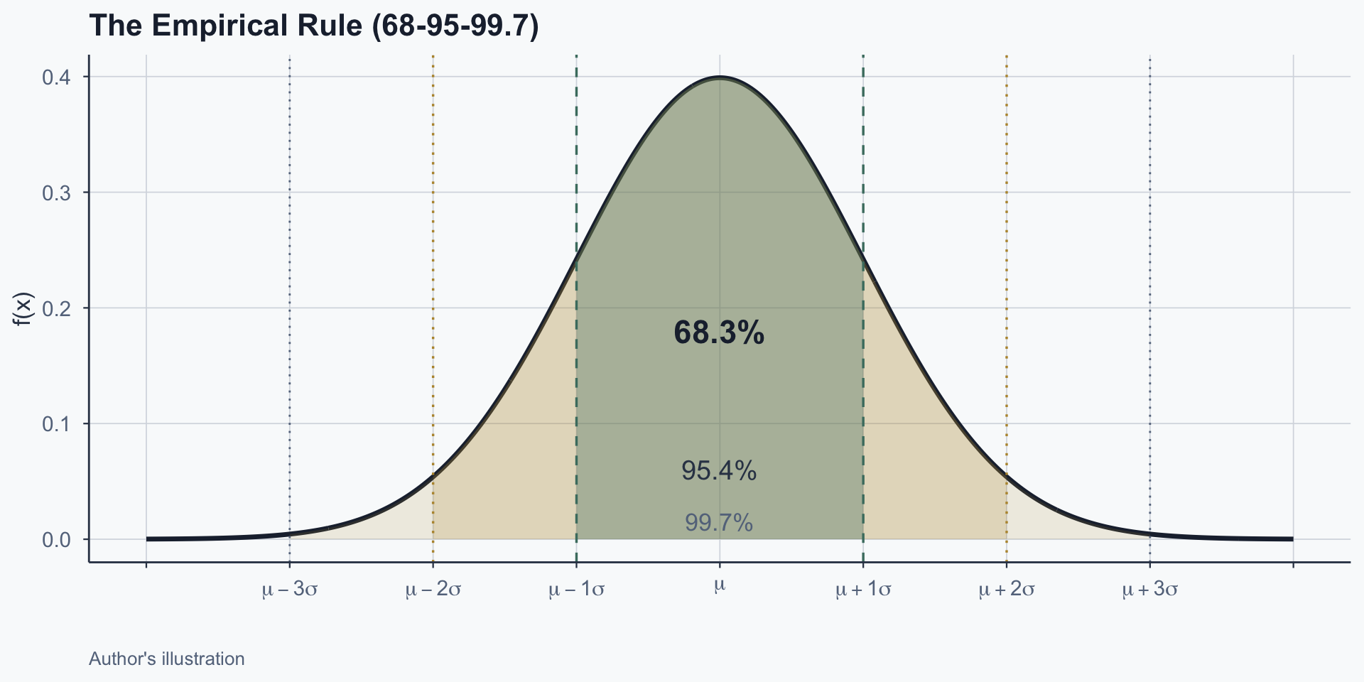
• Model: if data is approximately normal, two numbers (\(\mu\), \(\sigma\)) plus the 68-95-99.7 rule give you most of the picture
• Communicate: PMF, PDF, and CDF are the shared language for describing how variables behave

Next: we’ll use these tools in R with pnorm, qnorm, and dnorm.