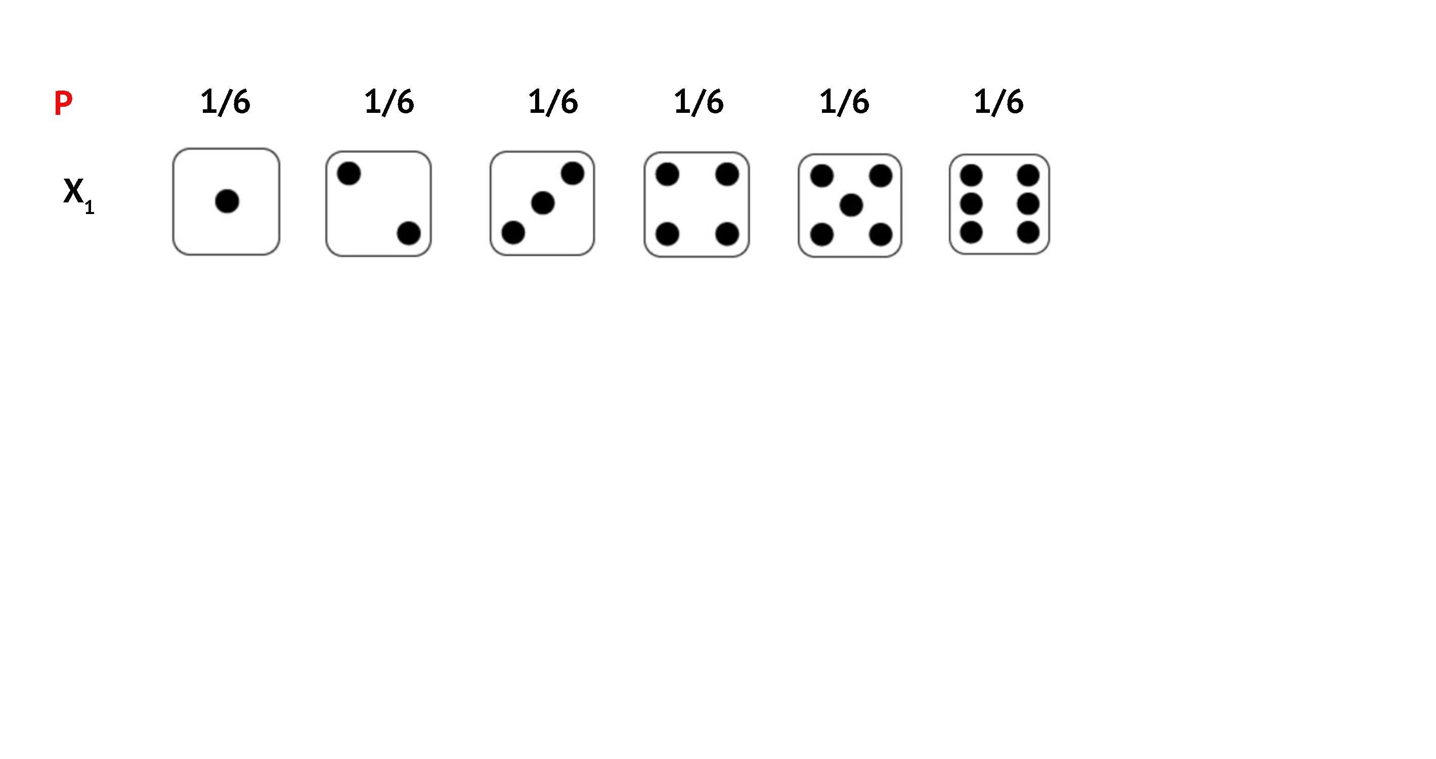
Multiplication Rule
For independent events:
\[P(A \text{ and } B) = P(A) \times P(B)\]
Events are independent when one outcome does not affect the other
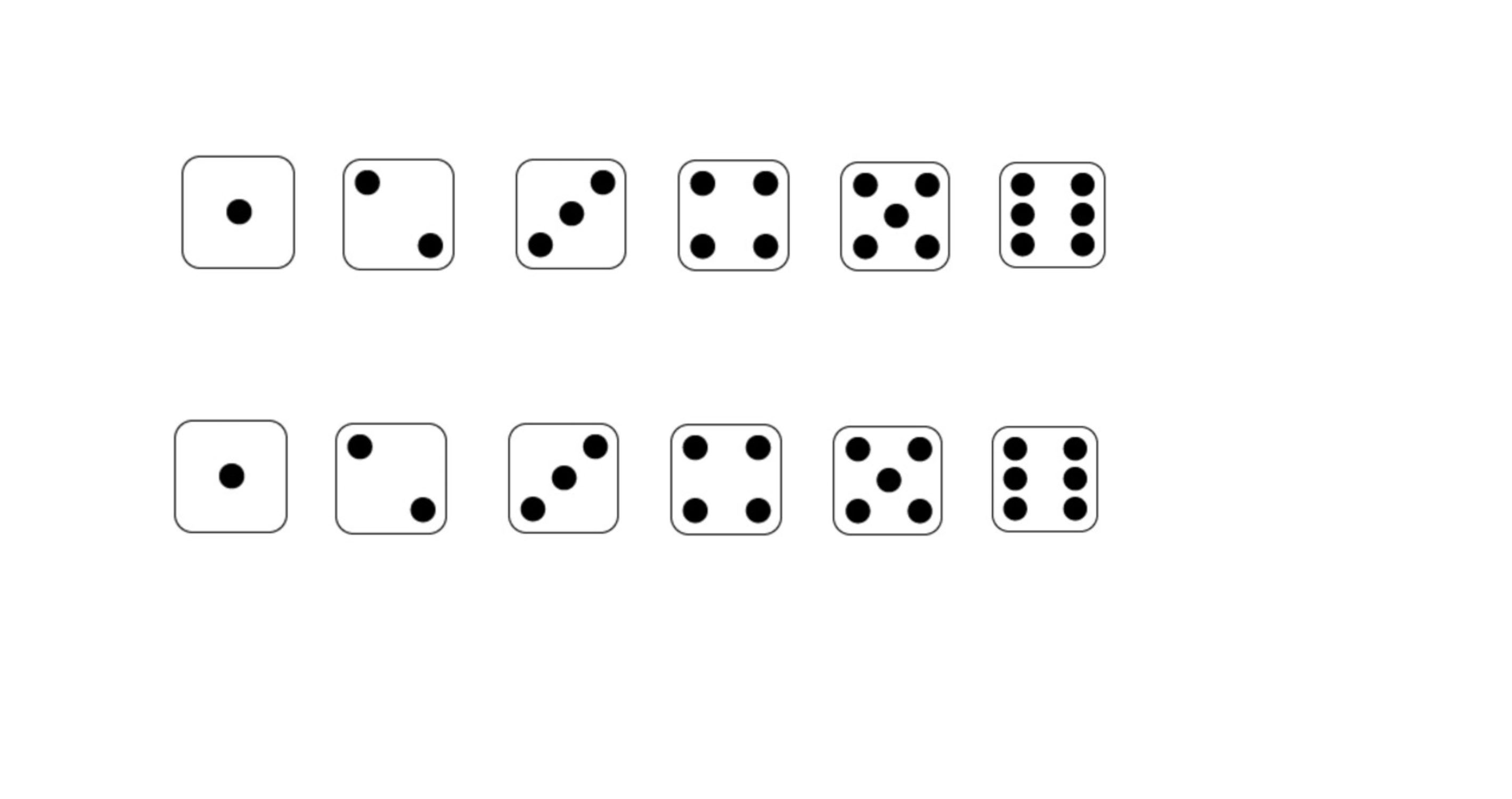
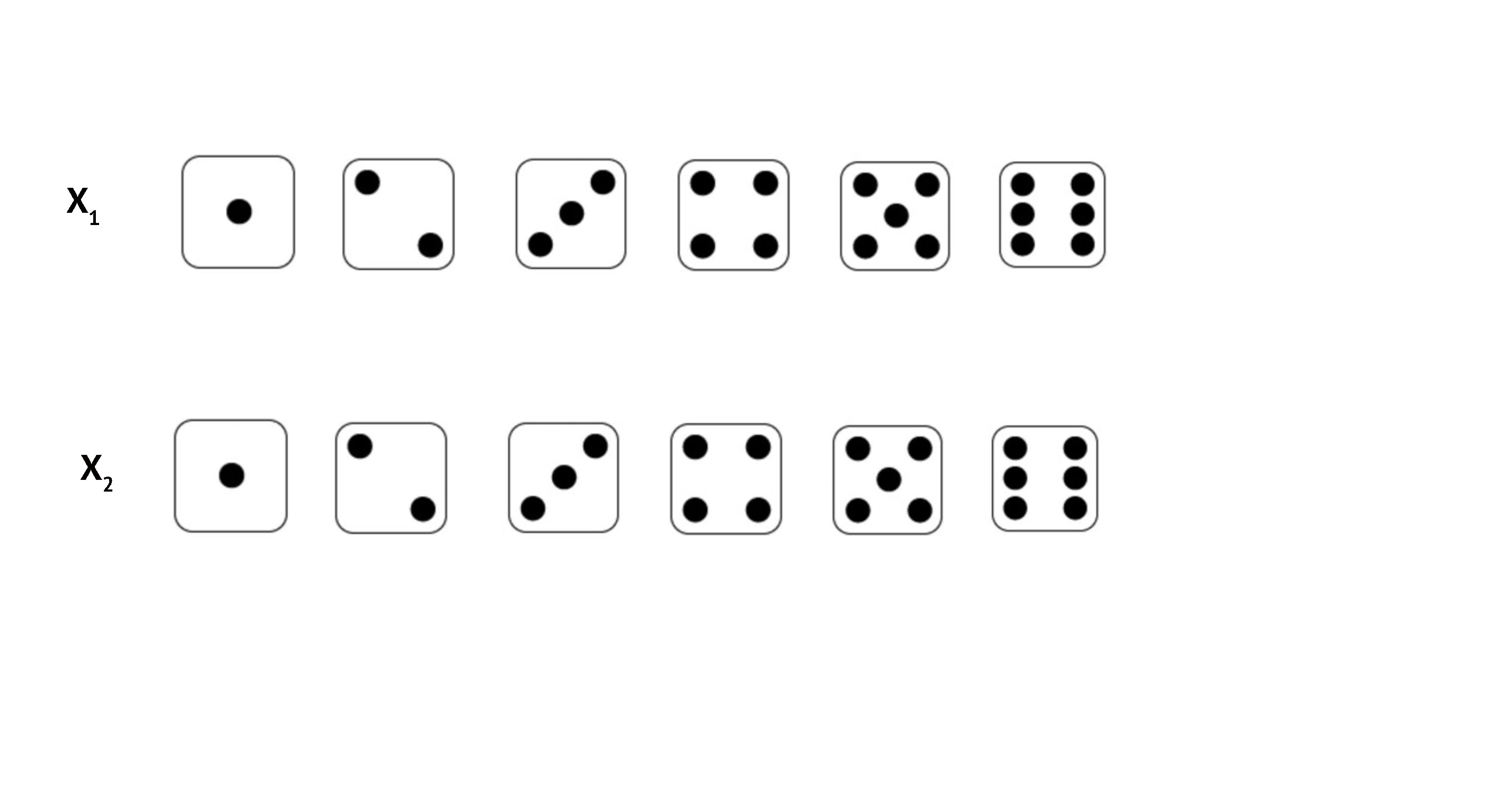
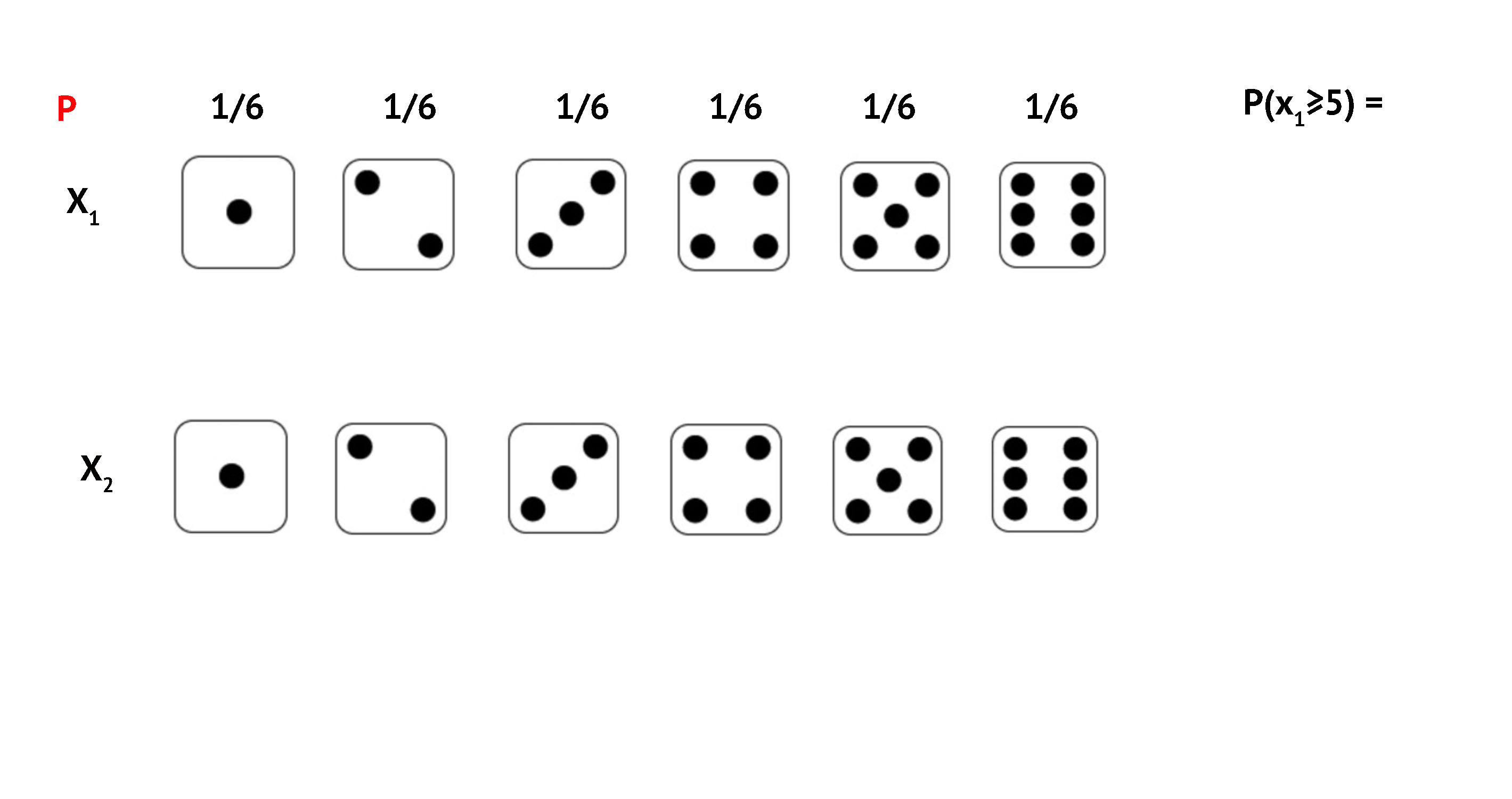
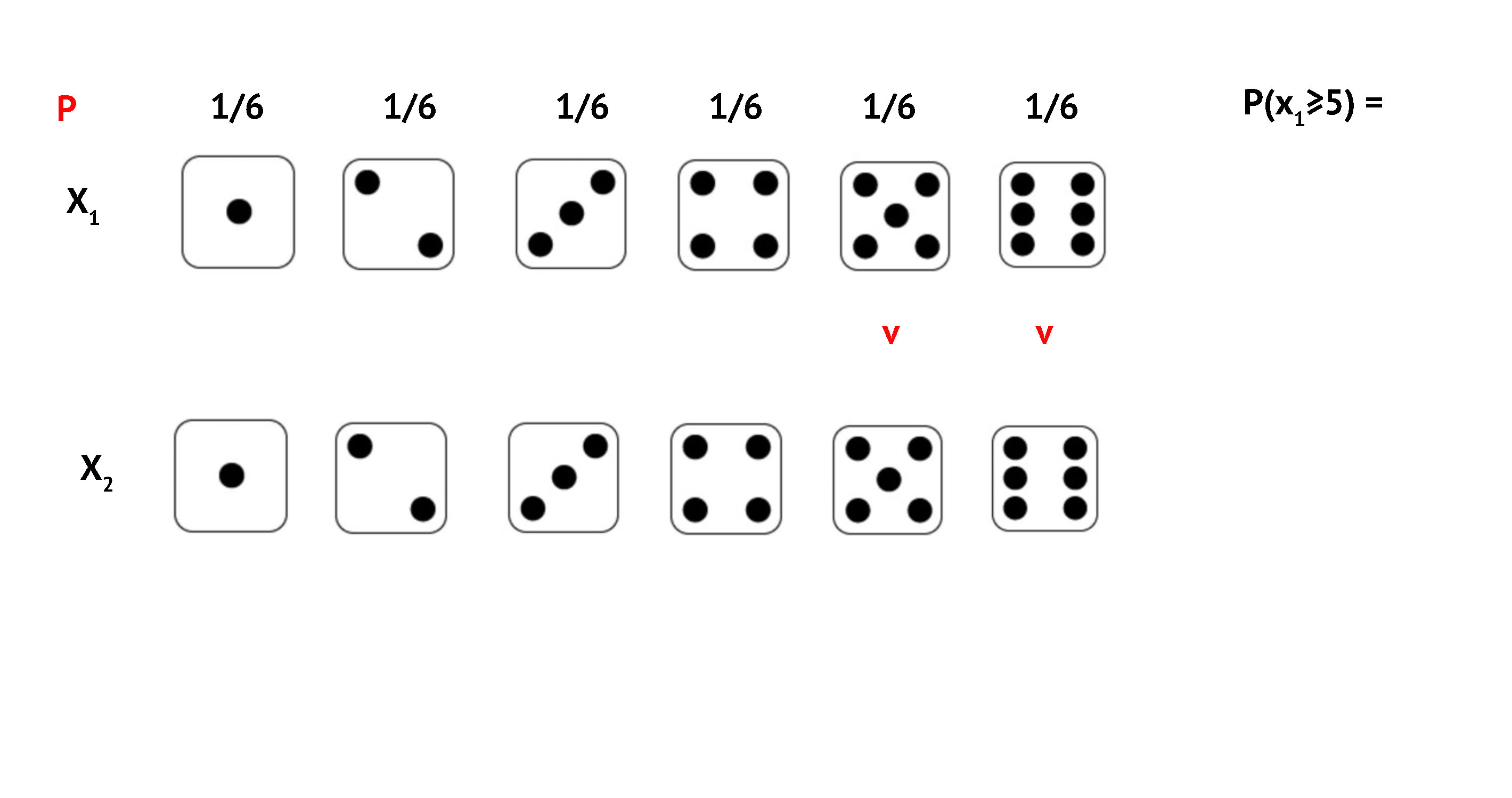
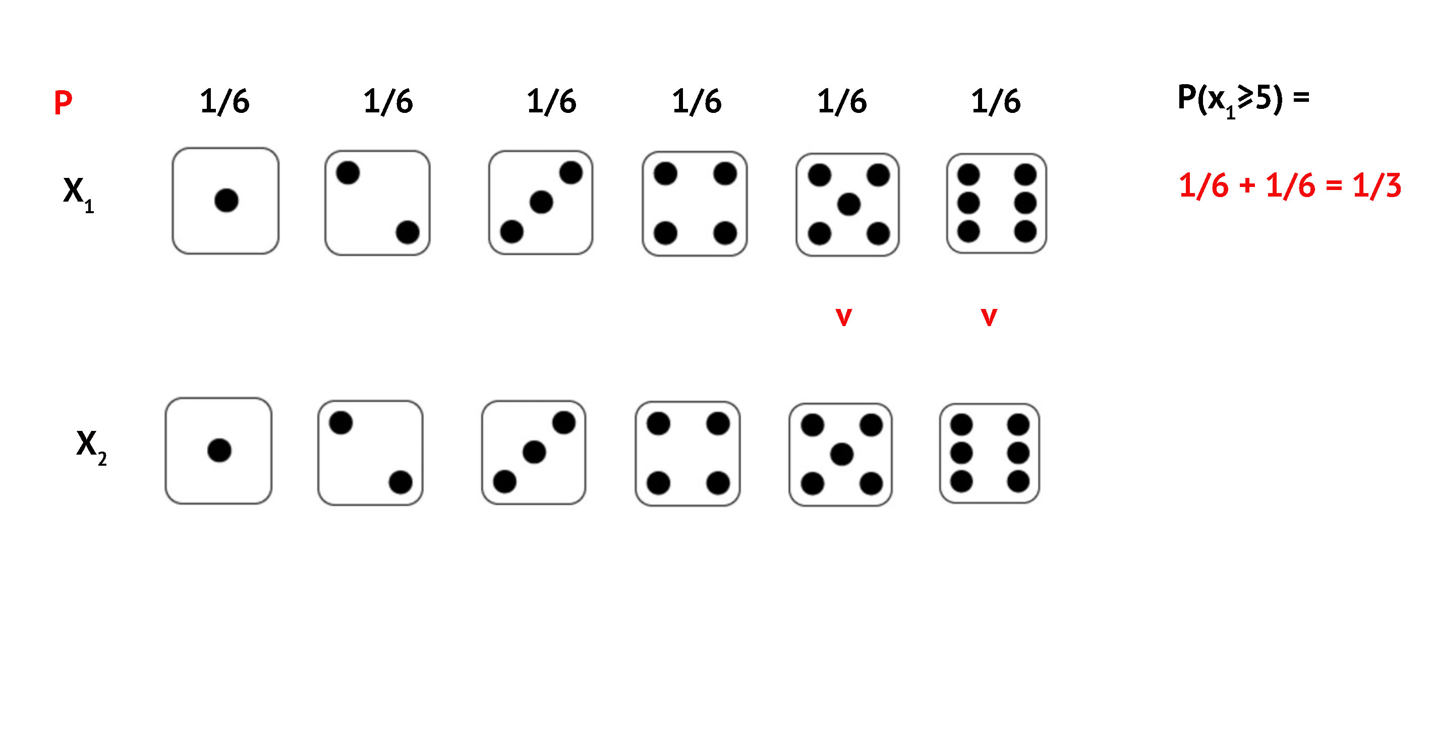
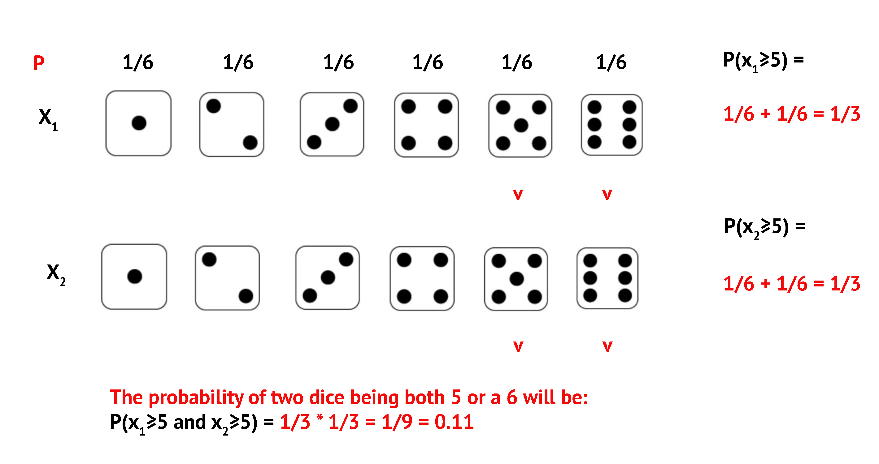
Example 3: Roll two dice. What is \(P(\text{both} \geq 5)\)?
Example 3: Both Dice \(\geq\) 5
![]()
Example 3: Both Dice \(\geq\) 5
![]()
Example 3: Both Dice \(\geq\) 5
![]()
Example 3: Both Dice \(\geq\) 5
![]()
Example 3: Both Dice \(\geq\) 5
![]()
Example 3: Both Dice \(\geq\) 5
![]()
Example 3: Both Dice \(\geq\) 5
![]()
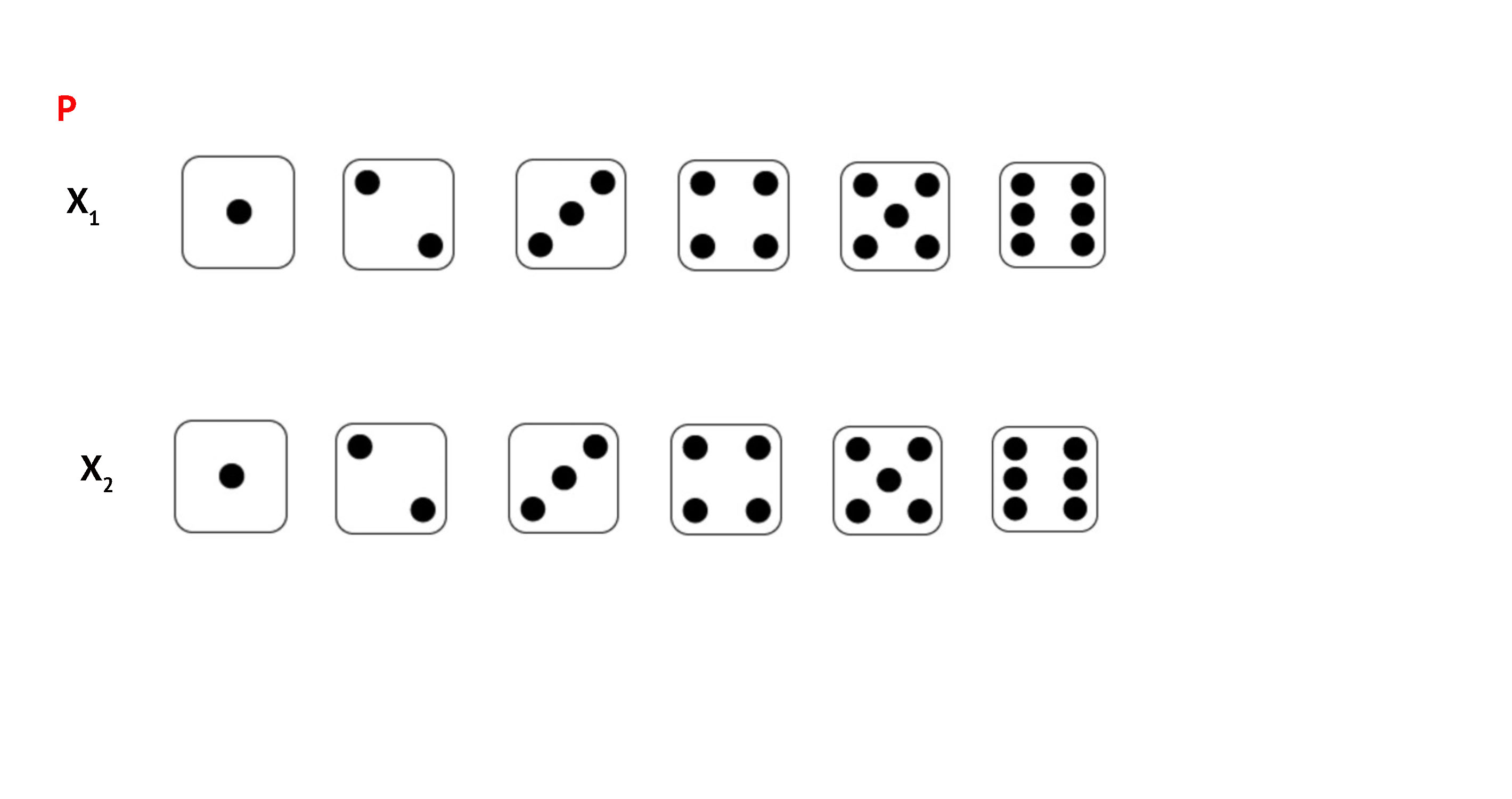
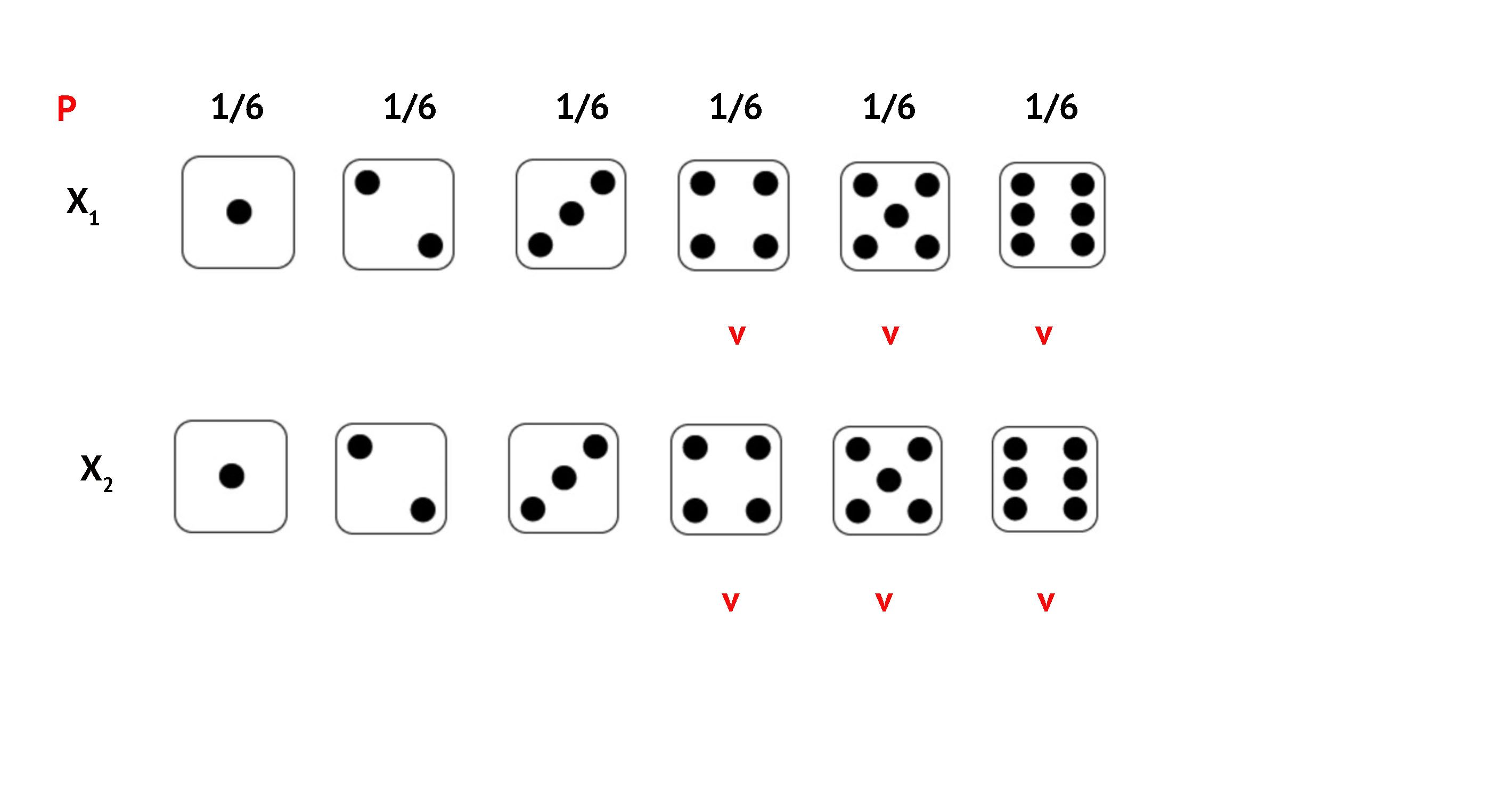
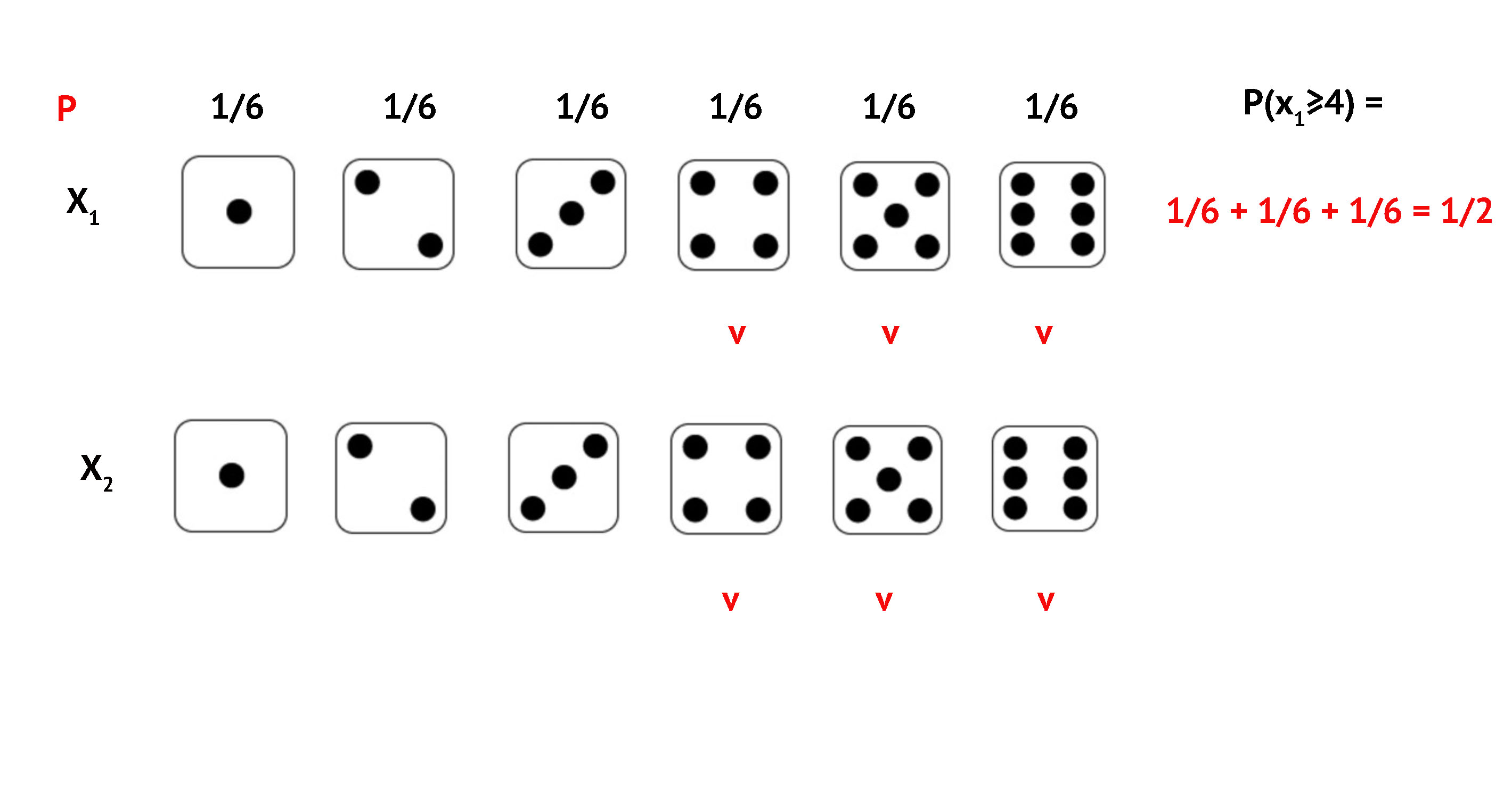
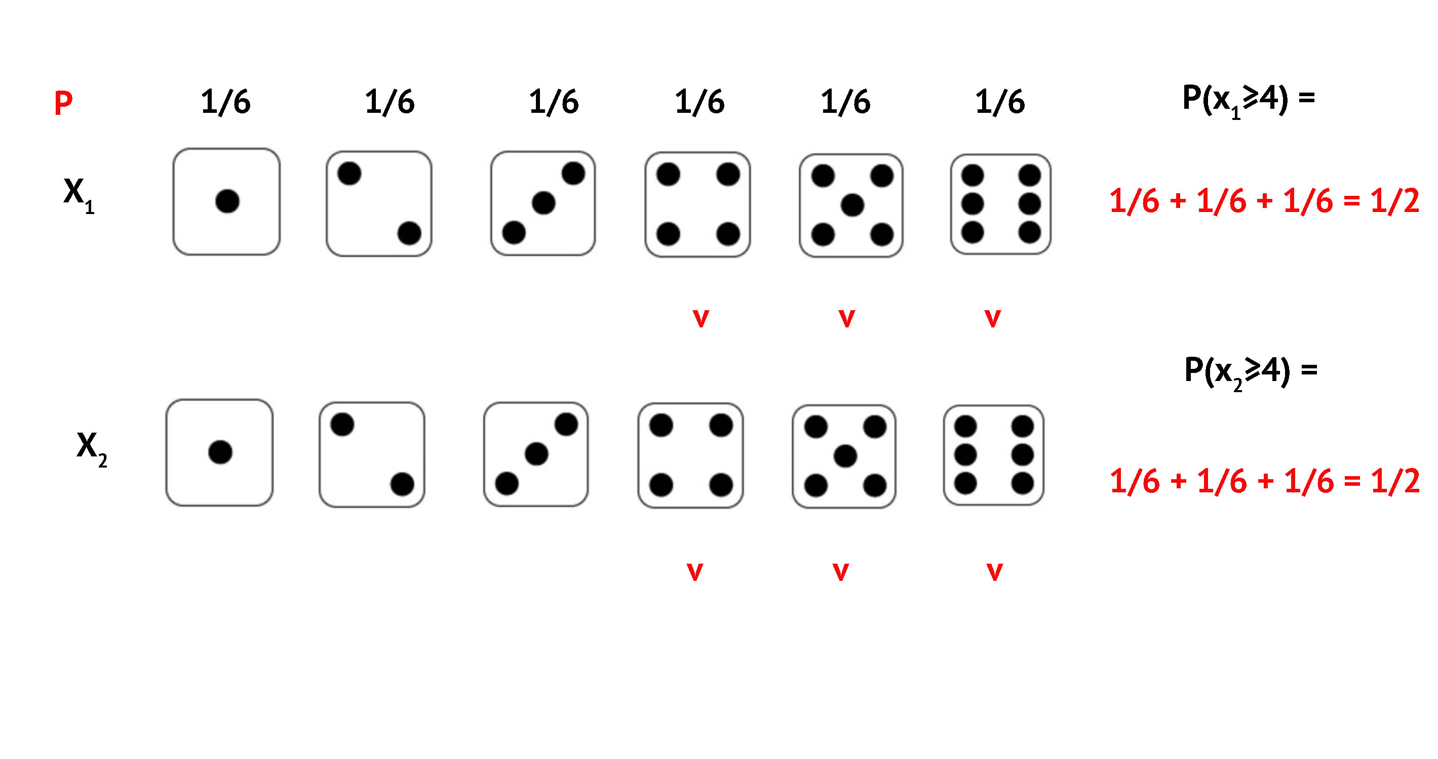
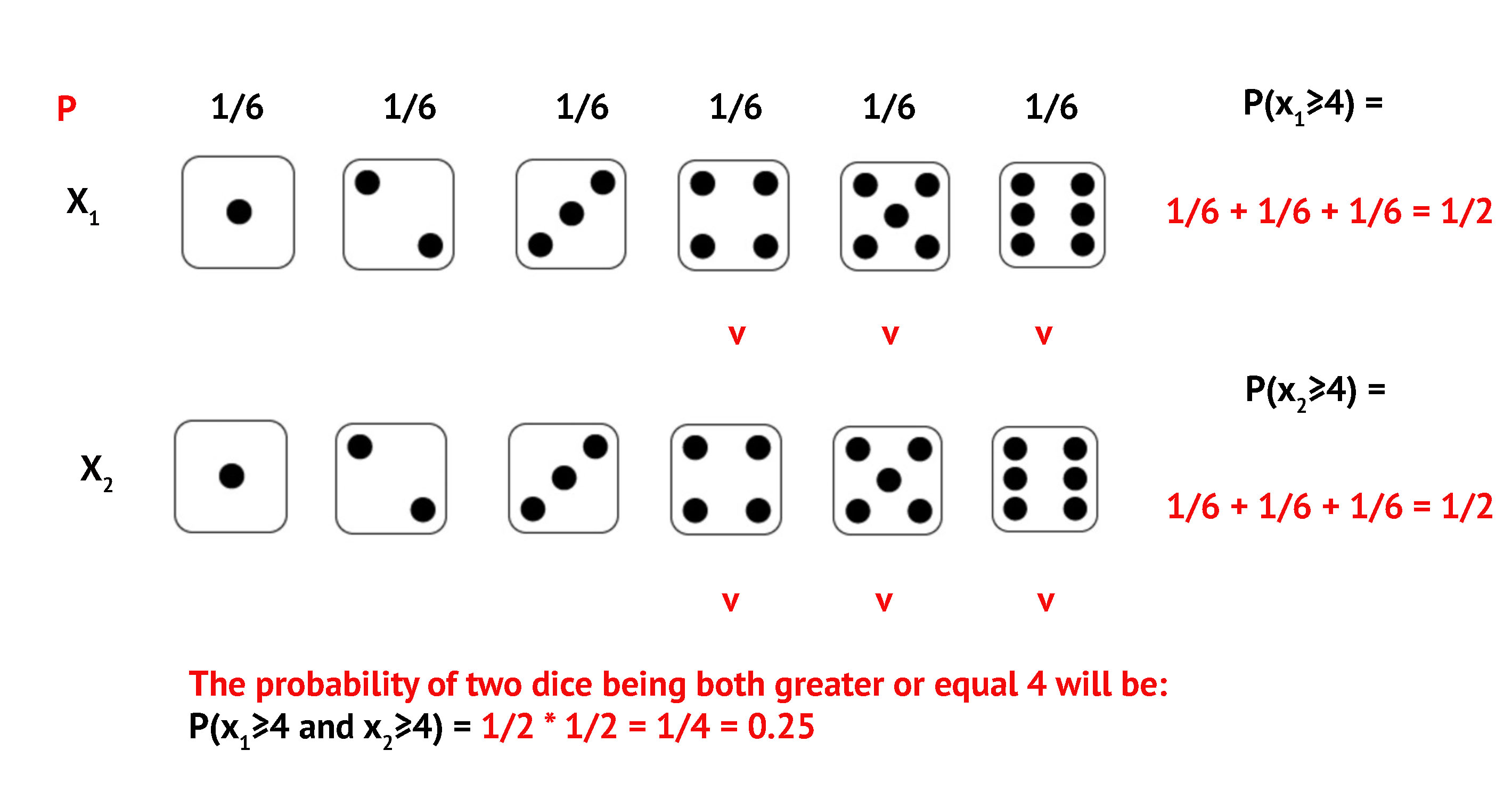
Exercise: Both Dice \(\geq\) 4
\(P(\text{both} \geq 4)\)?
![]()
Exercise: Both Dice \(\geq\) 4
![]()
Exercise: Both Dice \(\geq\) 4
![]()
Exercise: Both Dice \(\geq\) 4
![]()
Exercise: Both Dice \(\geq\) 4
![]()
Exercise: Both Dice \(\geq\) 4
![]()
Exercise: Both Dice \(\geq\) 4
![]()
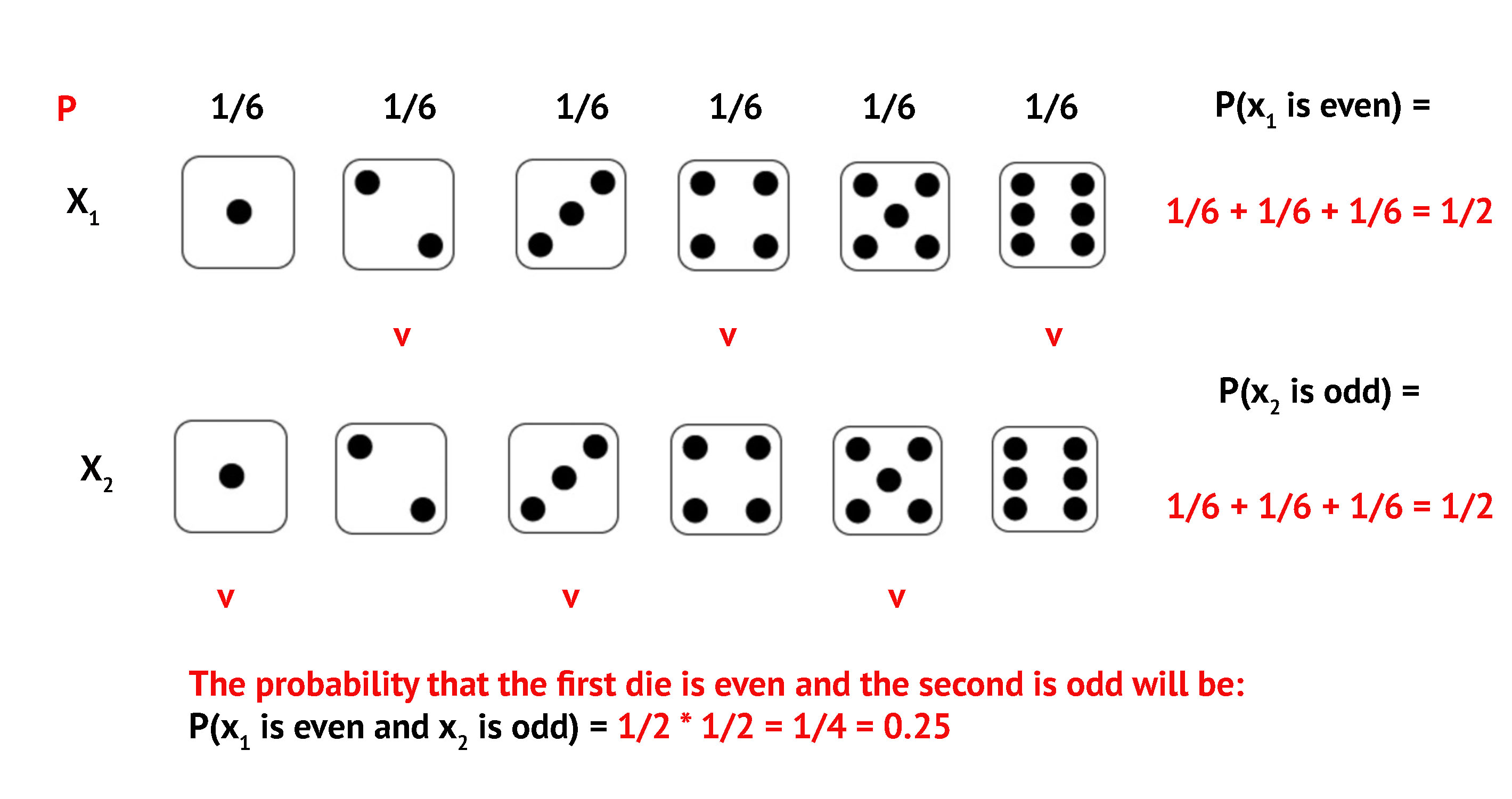
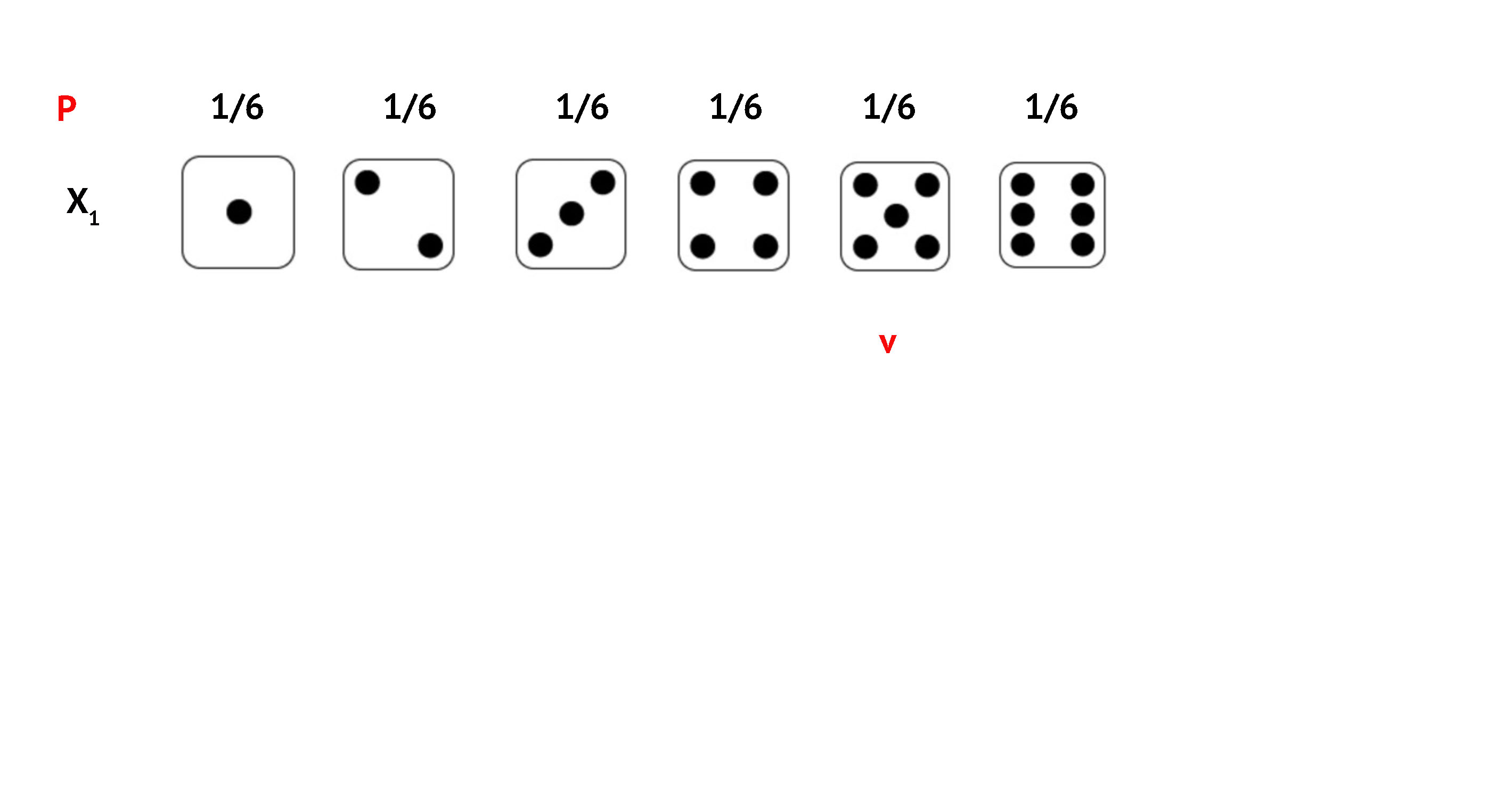
At Least One Even Number
Example 5: Roll two dice. \(P(\text{at least one even})\)?
Four possibilities:
- Even and Odd
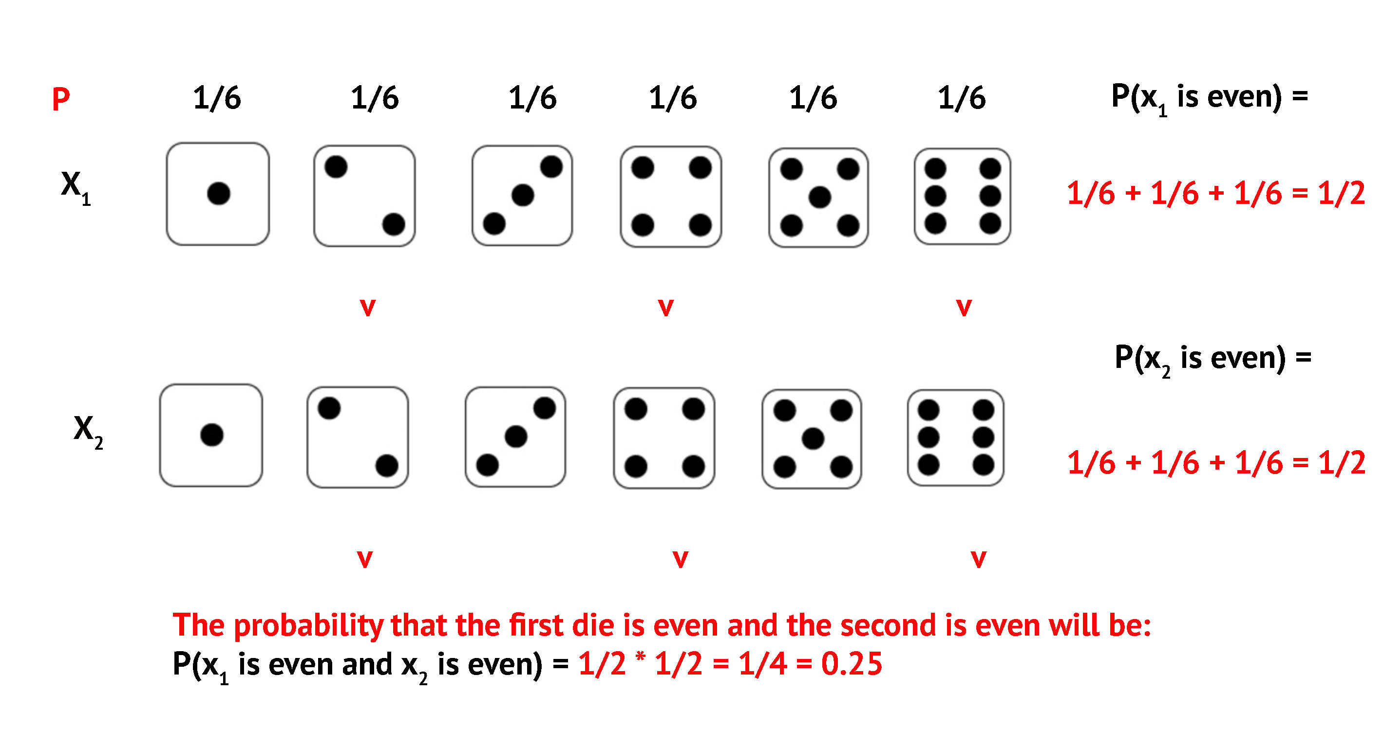
- Even and Even
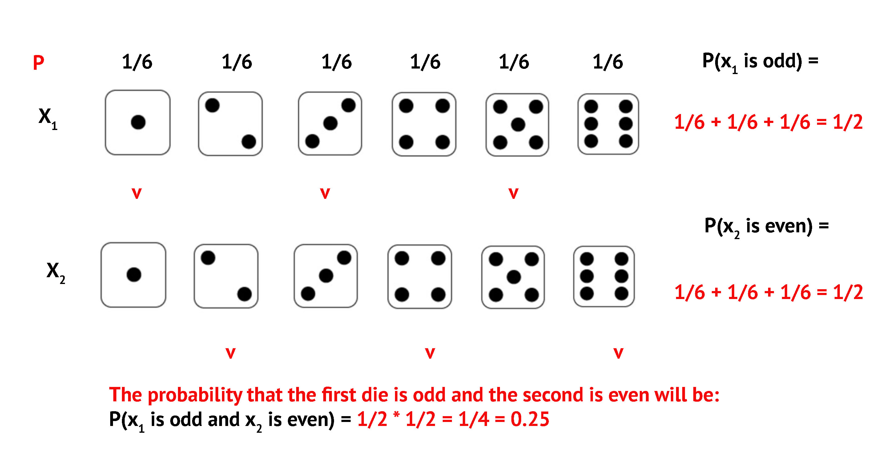
- Odd and Even
- Odd and Odd
At Least One Even: Option 1
Even and Odd: \(P = 1/2 \times 1/2 = 1/4\)
![]()
At Least One Even: Option 2
Even and Even: \(P = 1/2 \times 1/2 = 1/4\)
![]()
At Least One Even: Option 3
Odd and Even: \(P = 1/2 \times 1/2 = 1/4\)
![]()
At Least One Even: Result
Three favorable outcomes, each with \(P = 1/4\):
\[P(\text{at least one even}) = \frac{1}{4} + \frac{1}{4} + \frac{1}{4} = \frac{3}{4}\]
The Complement Rule
We can calculate any probability using its complement:
\[P(A) = 1 - P(A^C)\]
- \(A\) = at least one even number
- \(A^C\) = no even numbers (Odd and Odd) = \(1/4\)
\[P(A) = 1 - \frac{1}{4} = \frac{3}{4}\]
Exercise: P(Sum = 2)
Roll two dice. What is \(P(\text{sum} = 2)\)?
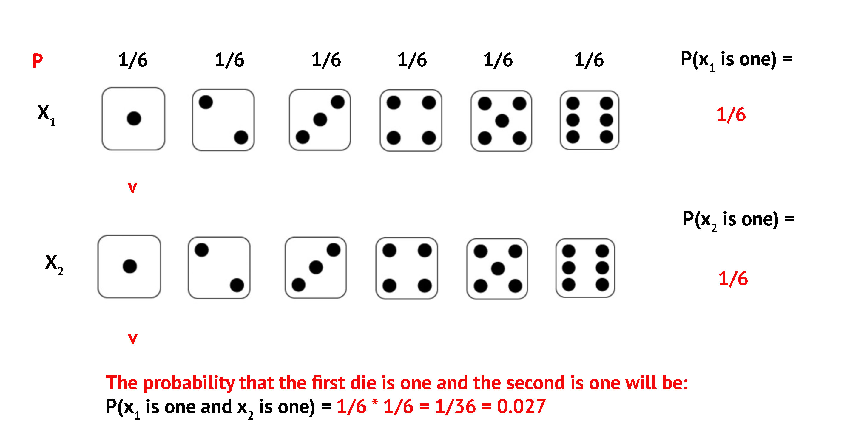
Only one way: both dice show 1
![]()
Exercise: P(Sum = 2)
\[P(\text{sum} = 2) = \frac{1}{6} \times \frac{1}{6} = \frac{1}{36}\]
Exercise: P(Sum = 7)
Roll two dice. What is \(P(\text{sum} = 7)\)?
Six ways to get 7:
| 1 |
1 |
6 |
1/36 |
| 2 |
6 |
1 |
1/36 |
| 3 |
2 |
5 |
1/36 |
| 4 |
5 |
2 |
1/36 |
| 5 |
3 |
4 |
1/36 |
| 6 |
4 |
3 |
1/36 |
Exercise: P(Sum = 7)
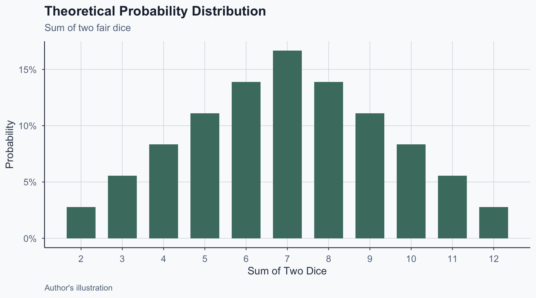
\[P(\text{sum} = 7) = 6 \times \frac{1}{36} = \frac{6}{36} = \frac{1}{6}\]
- Sum of 7 is the most likely outcome when rolling two dice
- This is because it has the most combinations
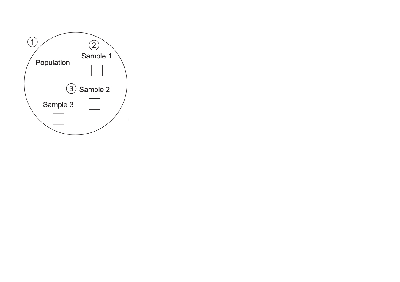
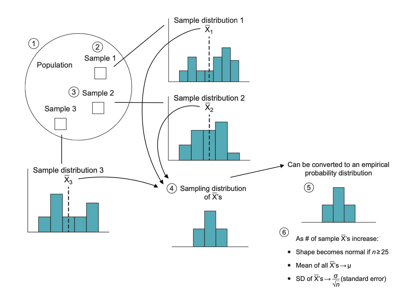
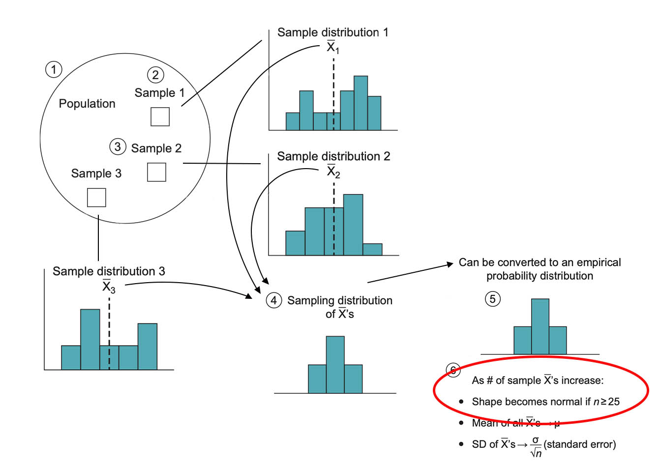
From Population to Samples
![]()
The logic of inferential statistics starts with a population
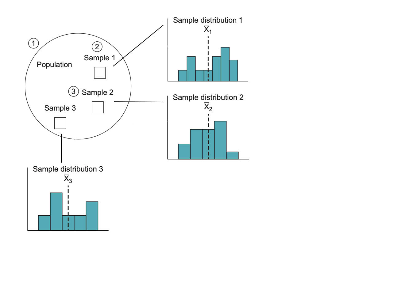
Drawing Repeated Samples
![]()
The researcher draws repeated samples: 1, 2, 3
Drawing Repeated Samples
![]()
The researcher draws repeated samples: 1, 2, 3
Drawing Repeated Samples
![]()
The researcher draws repeated samples: 1, 2, 3
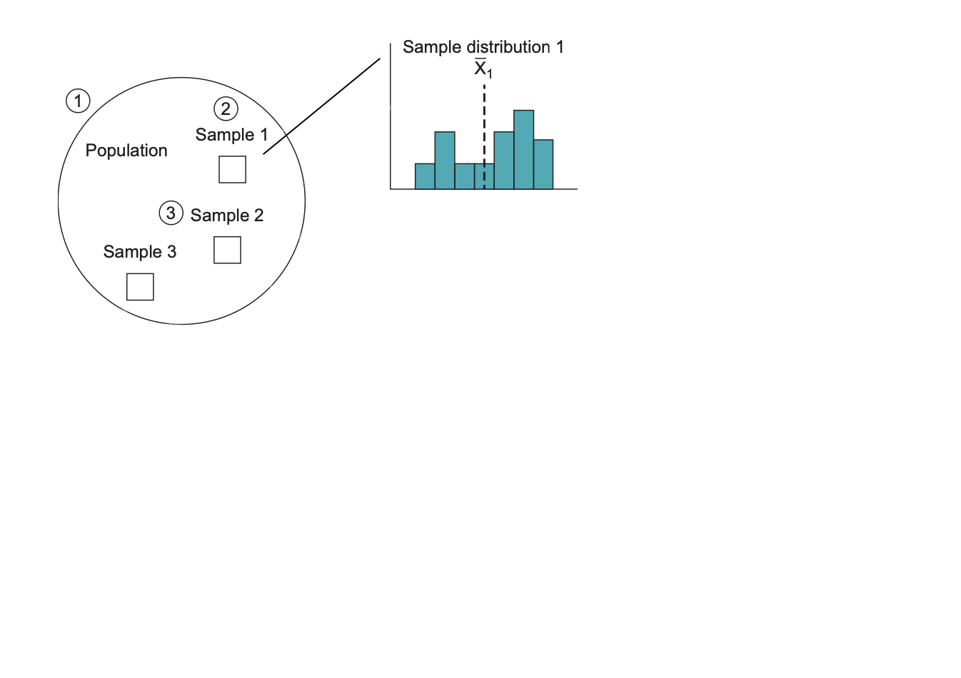
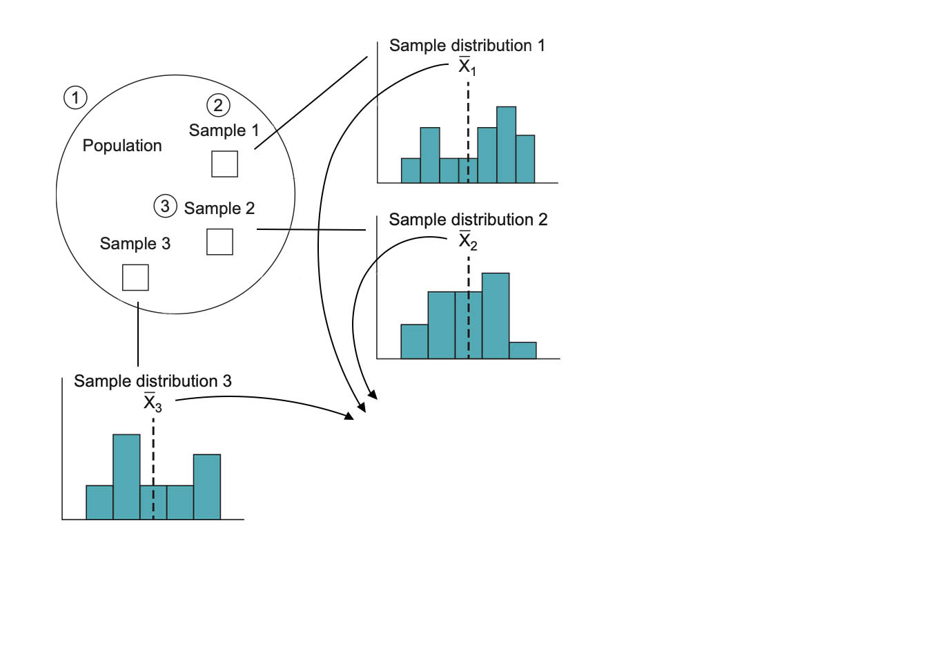
Calculating Sample Means
![]()
Each sample produces a sample mean
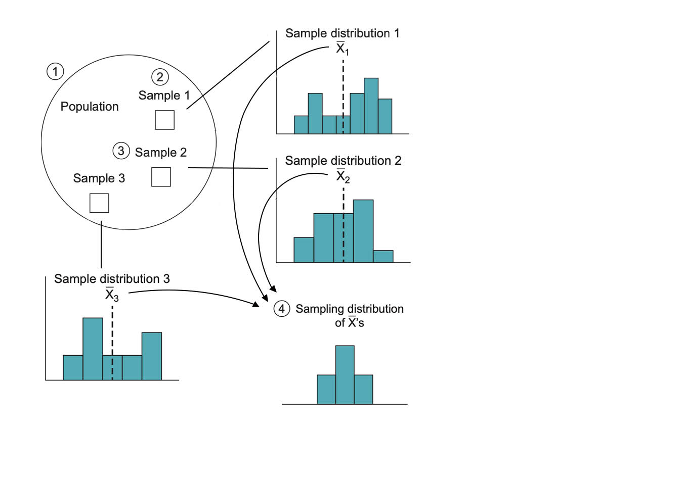
Sampling Distribution of Means
![]()
The sample means form a sampling distribution
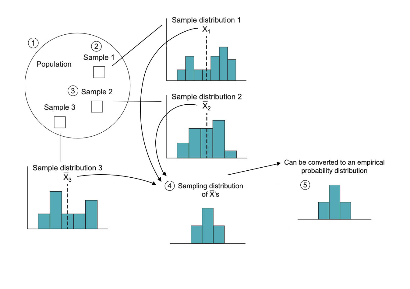
Sampling Distribution of Means
![]()
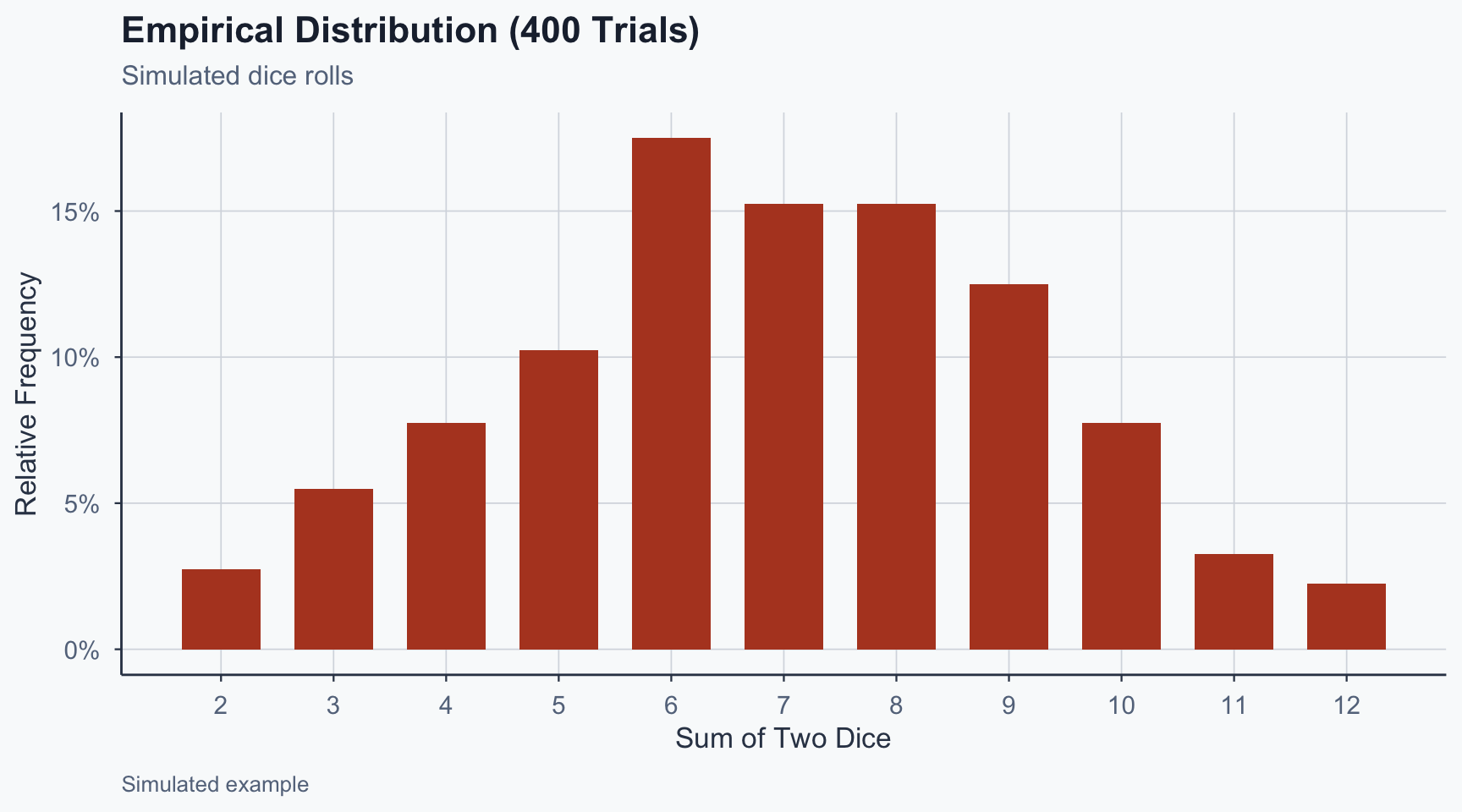
Can be converted to an empirical probability distribution
Sampling Distribution of Means
![]()
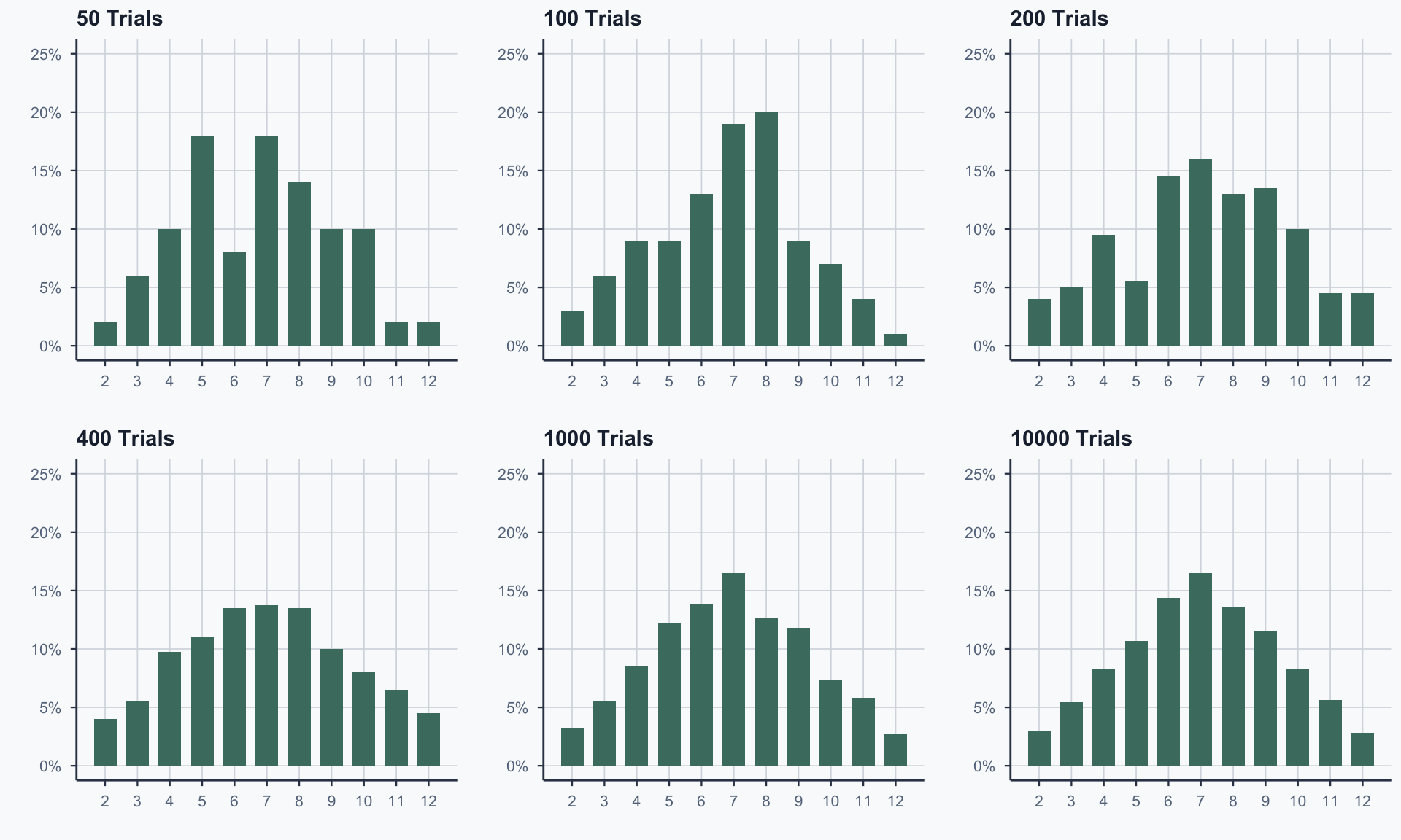
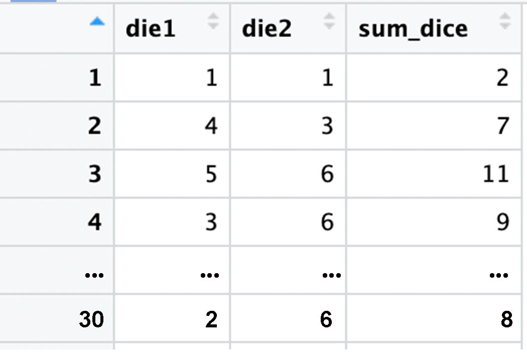
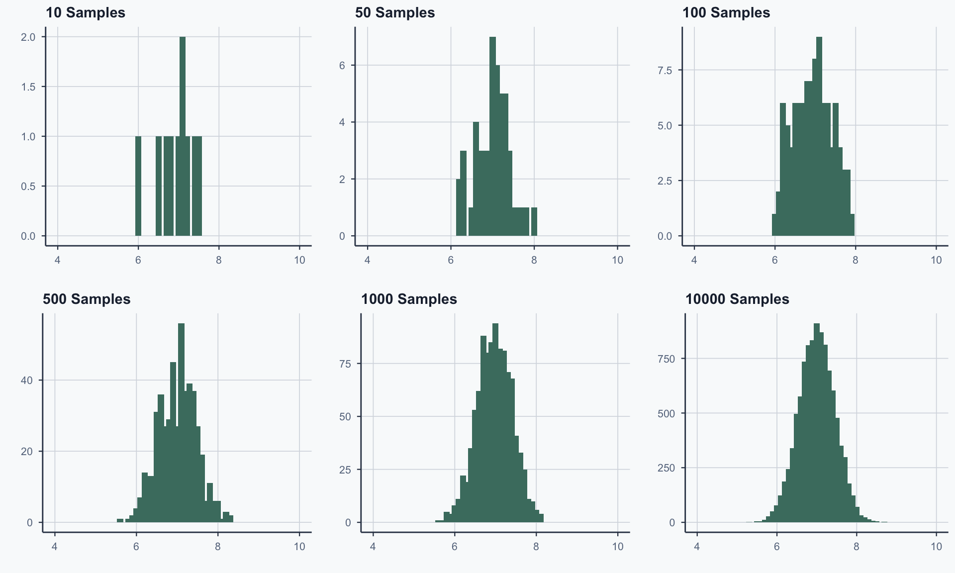
Simulation Setup
- Step 1: Roll two dice 30 times, calculate sum
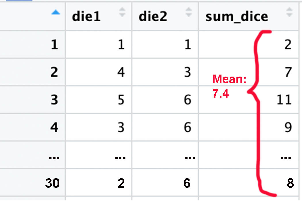
- Step 2: Compute the mean of those 30 sums
- Step 3: Repeat 10, 50, 100, 500, 1000, 10000 times
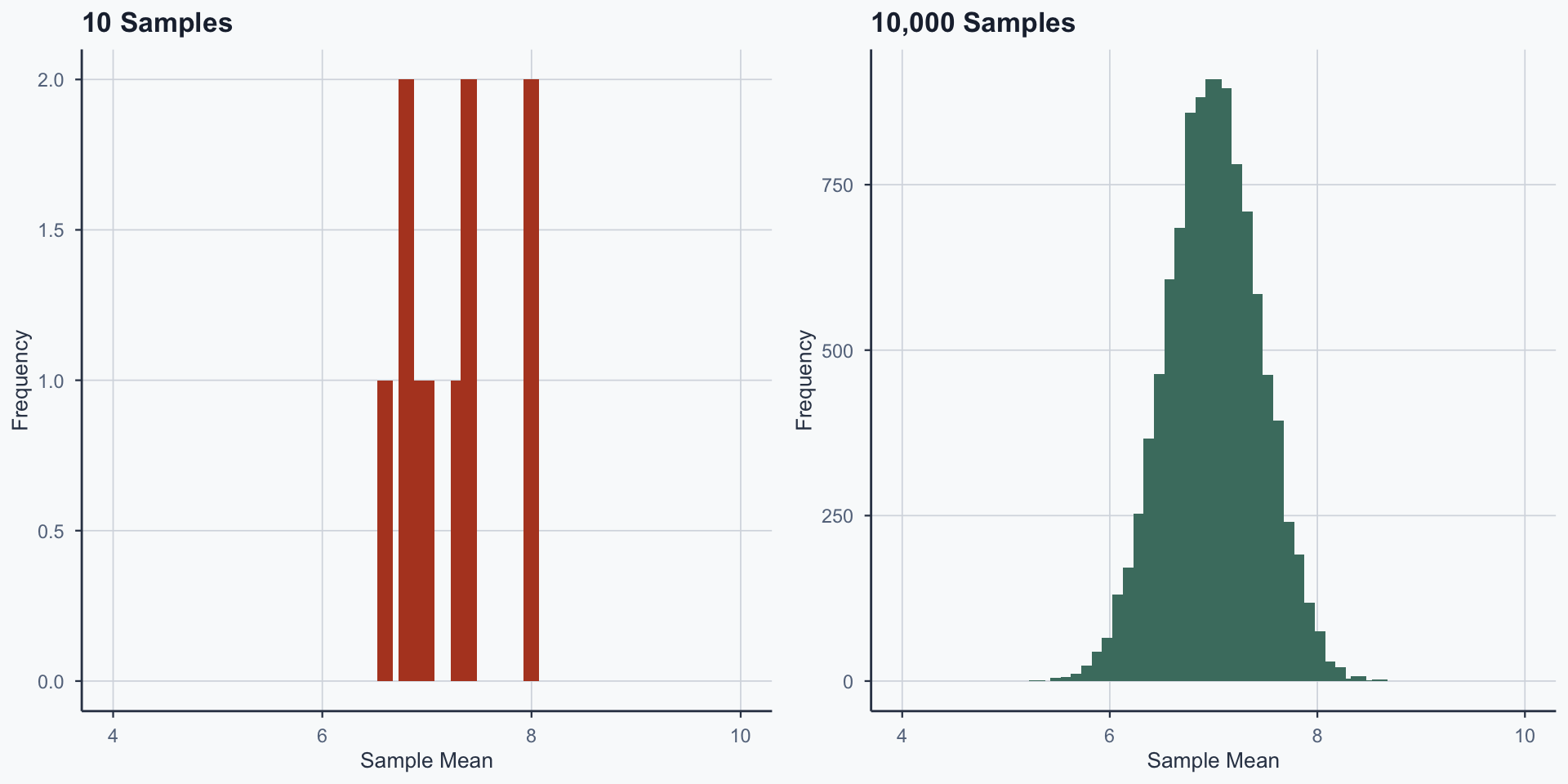
As we repeat more, the distribution of means takes shape
30 Dice Rolls (One Sample)
![]()
Sampling Distribution: 10 vs 10,000 Samples
![]()
Figure 4
Sampling Distribution Comparison
![]()
Figure 5
The Central Limit Theorem
The Central Limit Theorem (CLT) says something different from LLN:
- Take many samples of the same size from any population
- Compute the mean of each sample
- The distribution of those means is approximately normal (bell-shaped)
This holds regardless of the shape of the original distribution
- LLN: more trials → proportions converge to true probability
- CLT: distribution of sample means → normal distribution
LLN vs CLT: A Comparison
| About |
One long experiment |
Many repeated samples |
| What converges |
Proportions / averages → true value |
Distribution of sample means → normal |
| Requires |
More trials |
More samples (of fixed size) |
| Example |
10,000 die rolls → \(\bar{x} \to 3.5\) |
10,000 samples of 30 rolls → means form bell curve |
Summary
![]()
Real-World Application: Election Polling
A pollster surveys 1,000 voters. The candidate gets 52% support.
- Is the candidate truly ahead, or is this just sampling variability?
The CLT tells us: if we polled 1,000 voters many times, the sample proportions would form a bell curve around the true proportion
- If 52% is within the normal range of variation around 50% → we can’t be sure
- If 52% is far from what we’d expect under 50% → the lead is likely real
This is the foundation of margins of error and confidence intervals
Exercise 1: Your Turn
A bag contains 3 red, 2 blue, and 5 green marbles.
You draw one marble. Calculate:
- \(P(\text{red or blue})\)
- \(P(\text{not green})\)
- Are your answers to (1) and (2) the same? Why?
Hint: Think about which rule applies — addition or complement?
Exercise 1: Solution
\(P(\text{red or blue}) = \frac{3}{10} + \frac{2}{10} = \frac{5}{10} = \frac{1}{2}\)
\(P(\text{not green}) = 1 - P(\text{green}) = 1 - \frac{5}{10} = \frac{1}{2}\)
Yes — “red or blue” and “not green” describe the same event. The complement rule and the addition rule give the same answer.
Exercise 2: Your Turn
You draw two marbles with replacement.
What is \(P(\text{both green})\)?
Hint: Are the draws independent? Which rule applies?
Exercise 2: Solution
With replacement, draws are independent:
\[P(\text{both green}) = \frac{5}{10} \times \frac{5}{10} = \frac{25}{100} = \frac{1}{4}\]
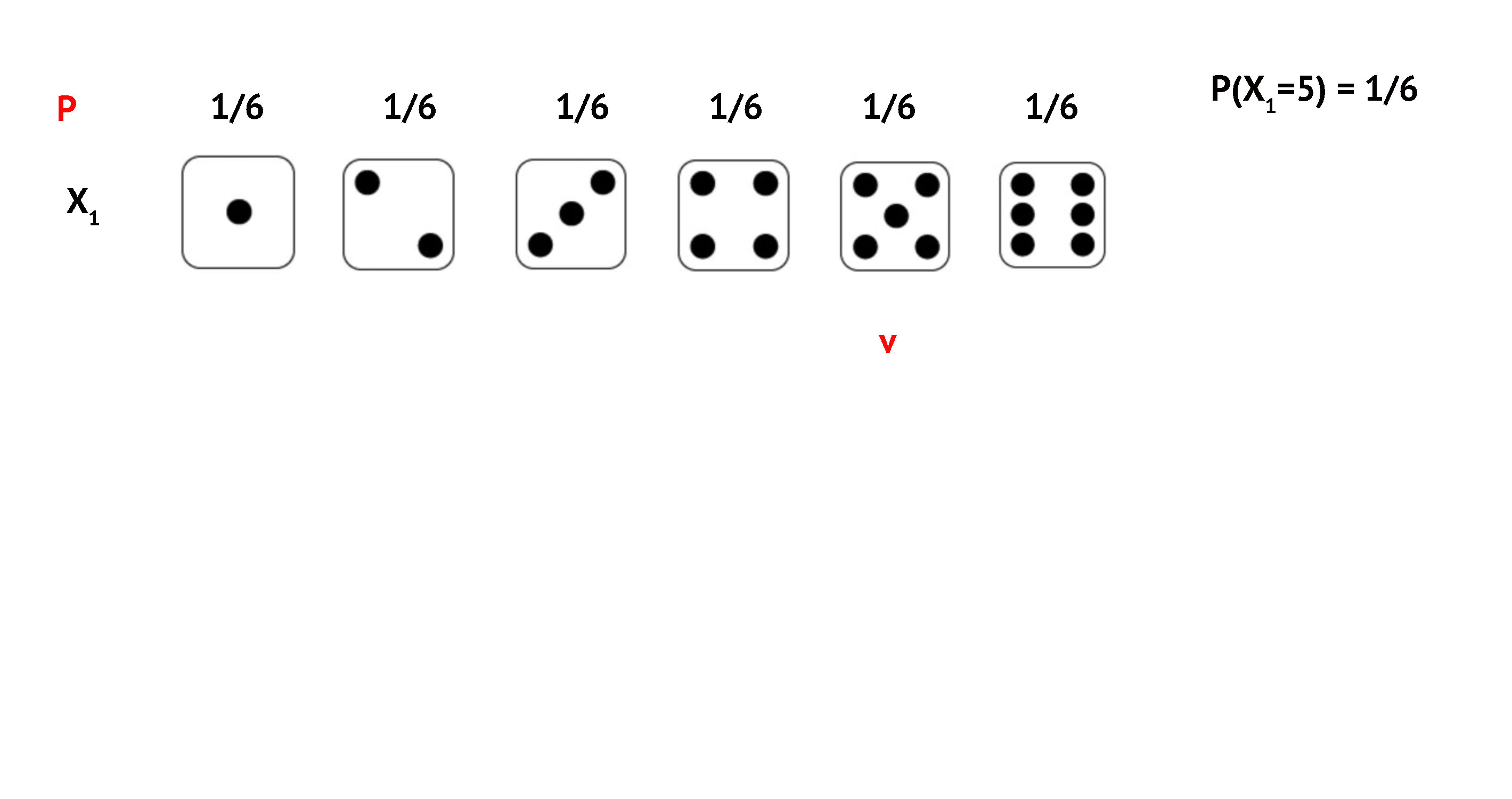
Exercise 3: 32 Consecutive Non-5 Rolls
What is \(P(\text{not 5 on all 32 throws})\)?
![]()
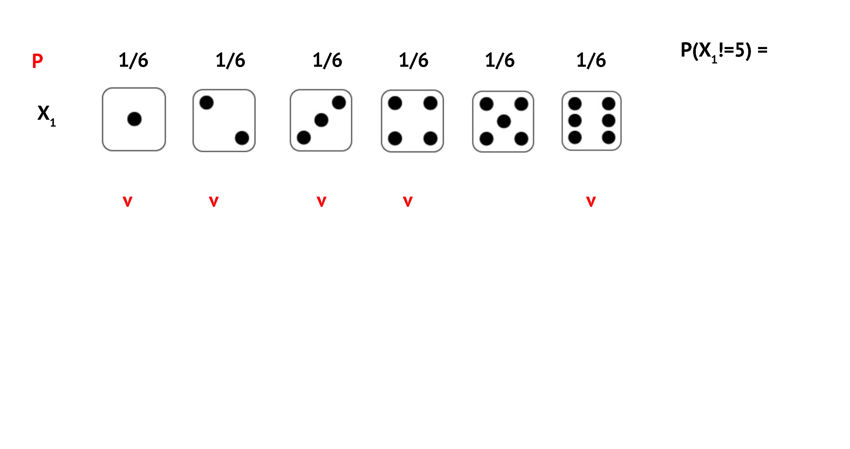
Exercise 3: 32 Non-5 Rolls
![]()
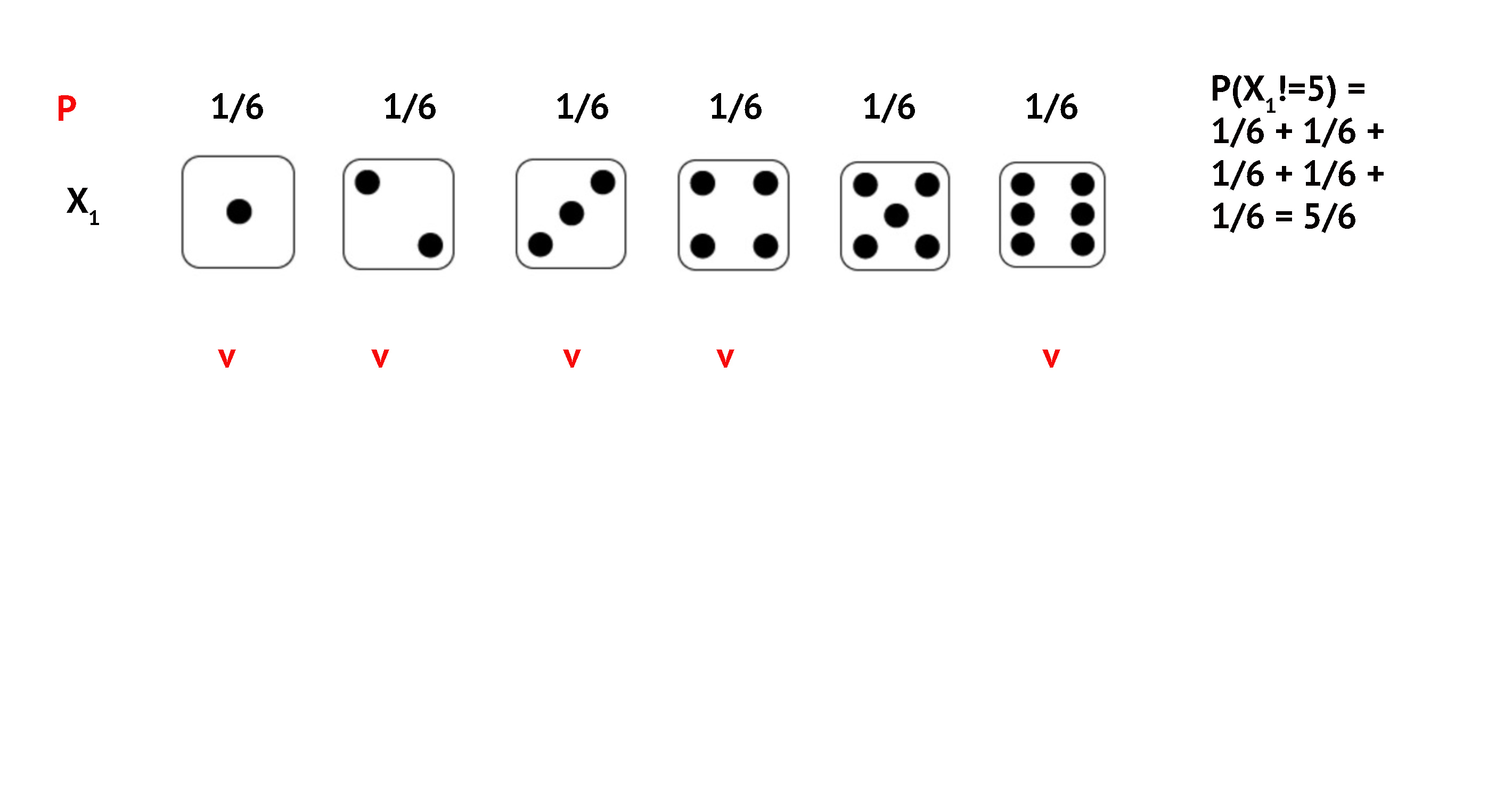
Exercise 3: 32 Non-5 Rolls
![]()
Exercise 3: 32 Non-5 Rolls
![]()
Exercise 3: 32 Non-5 Rolls
![]()
Exercise 3: 32 Non-5 Rolls
We multiply the probabilities (independent events):
\[P = \left(\frac{5}{6}\right)^{32} = 0.0029\]
- Each roll is independent — outcomes don’t affect each other
- We raise to the 32nd power, not multiply by 32
- This is a joint probability of 32 independent events