Statistical Analysis

Lecture 3: Descriptive Statistics

Bogdan G. Popescu

bogdan.popescu@johncabot.edu

John Cabot University

Why Summarize Data?

Raw datasets are long and messy. We need summaries that are:

Concise: easy to communicate
Informative: capture what matters
Comparable: across groups and time

Without summaries, we cannot test hypotheses or compare groups – the core of statistical inference

From Description to Inference

%%{init:{"flowchart":{"useMaxWidth":true,"nodeSpacing":50,"rankSpacing":50},"themeVariables":{"fontSize":"22px"},"width":1150,"height":650}}%%
flowchart LR
  A[Raw Data] --> B[Descriptive<br/>Statistics]
  B --> C[Identify<br/>Patterns]
  C --> D[Formulate<br/>Hypotheses]
  D --> E[Inferential<br/>Statistics]

Two Ways to Summarize

Graphical summaries

Bar charts, histograms, density plots, boxplots

Numerical summaries

Central tendency: mode, median, mean
Dispersion: range, variance, standard deviation

A good summary always reports both center and spread

Frequency Distributions

Frequency table: counts of each value/category
Let $f_k$ = count for category $k$, $n$ = sample size

Relative frequency (proportion):

\[p_k = \frac{f_k}{n}\]

Measures of Central Tendency

Central Tendency

Describe the typical case in a dataset

Mode: most frequent value
Median: middle value (robust to outliers)
Mean: arithmetic average (uses all values)

Which one you report depends on the shape of the data and the research question

Mode

The most frequently occurring value
Defined only by frequency, not distance
May be absent or have multiple modes

\[[1, 3, 6, 6, 6, 6, 7, 7, 12, 12, 17]\]

The mode is 6 (occurs four times)

Visualizing the Mode

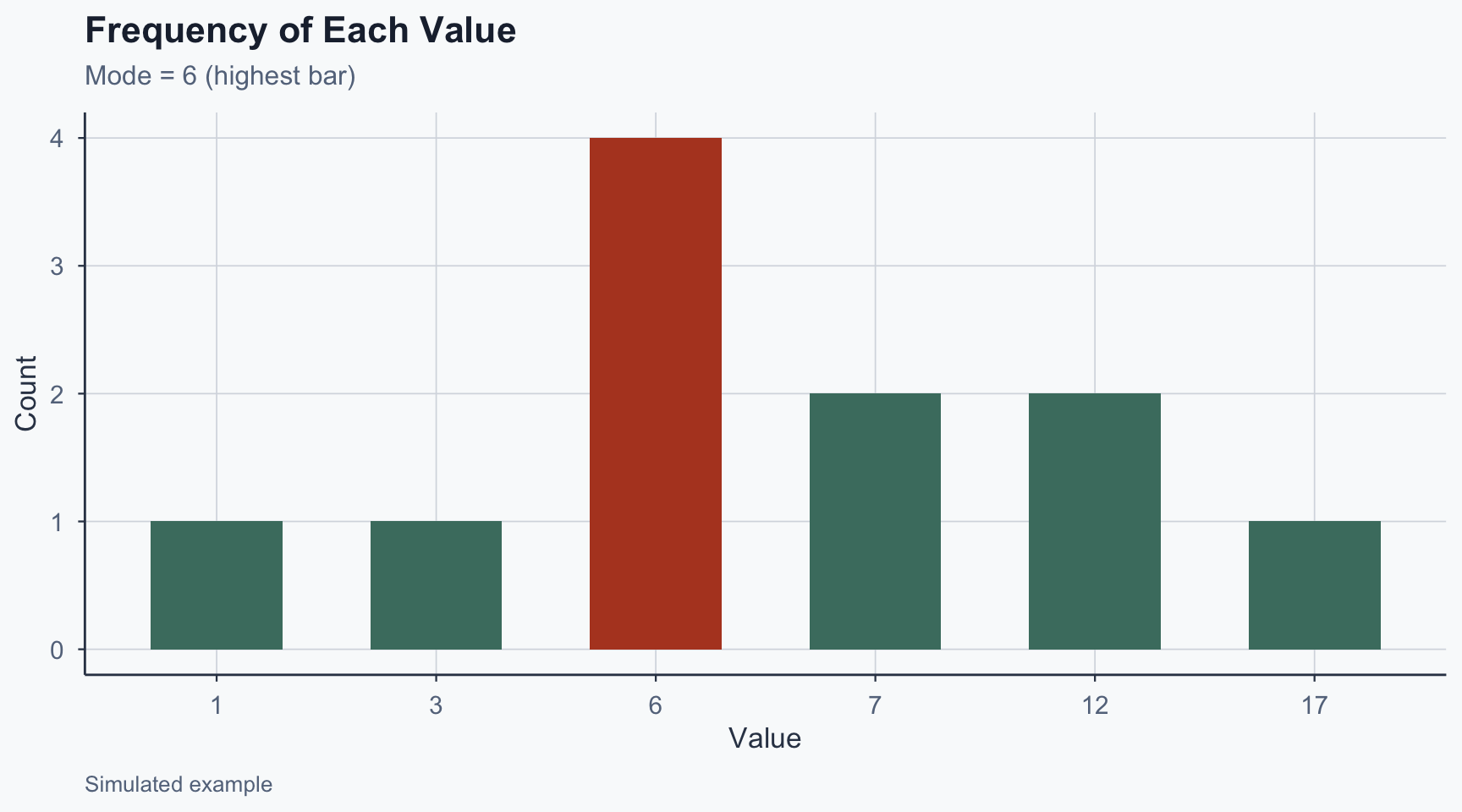
Figure 1

Median

The middle value in an ordered dataset
Requires observations to be ranked first
Resistant to outliers – preferred for skewed data

If $n$ is odd: $\quad\text{median} = x_{(n+1)/2}$

If $n$ is even: $\quad\text{median} = \frac{x_{n/2} + x_{(n/2)+1}}{2}$

Median: Odd $n$ Example

\[[1, 2, 2, \mathbf{3}, 4, 7, 9] \quad (n = 7)\]

\[\text{median} = x_{(7+1)/2} = x_4 = \mathbf{3}\]

Median: Even $n$ Example

\[[7, 3, 1, 2, 5, 6] \quad\rightarrow\quad [1, 2, 3, 5, 6, 7] \quad (n = 6)\]

\[\text{median} = \frac{x_3 + x_4}{2} = \frac{3 + 5}{2} = \mathbf{4}\]

Mean

The average of all values
Uses all observations – sensitive to outliers

\[\bar{x} = \frac{1}{n}\sum_{i=1}^{n} x_i\]

Example: $[4, 1, 7]$

\[\bar{x} = \frac{4 + 1 + 7}{3} = \frac{12}{3} = \mathbf{4}\]

When Does the Choice Matter?

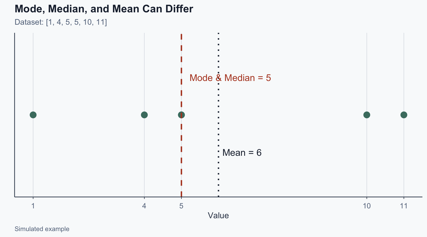
Figure 2

Choosing the Right Measure

Situation	Best measure	Why
Skewed income data	Median	Resistant to outliers
Symmetric exam scores	Mean	Uses all information
Categorical (party ID)	Mode	Only option
Small sample, outliers	Median	More stable

Exercise: Central Tendency

\[[1, 4, 5, 5, 10, 11]\]

Mode: 5 (most frequent)
Median: $\frac{x_3 + x_4}{2} = \frac{5+5}{2} = 5$
Mean: $(1+4+5+5+10+11)/6 = 36/6 = 6$

Note: mean $\neq$ median – the right tail pulls the mean up

Measures of Dispersion

Why Dispersion Matters

Two datasets can have the same mean but tell very different stories

Country A: incomes of $49k, $50k, $51k (low spread)
Country B: incomes of $10k, $50k, $90k (high spread)

Without measuring spread, we cannot assess uncertainty or test whether group differences are real

Visualizing Spread

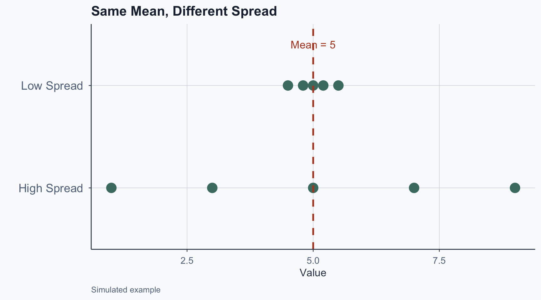
Figure 3

Range

Simplest measure: $\text{Range} = Y_{\max} - Y_{\min}$
Uses only two values – very sensitive to outliers

Better measures use all observations: variance and standard deviation

Variance

Sample variance (denominator $n - 1$):

\[s^2 = \frac{\sum_{i=1}^{n}(Y_i - \bar{Y})^2}{n-1}\]

Population variance (denominator $N$):

\[\sigma^2 = \frac{\sum_{i=1}^{N}(Y_i - \mu)^2}{N}\]

Standard Deviation

Square root of variance – same units as data
Easier to interpret than variance

Sample: $\quad s = \sqrt{\frac{\sum_{i=1}^{n}(Y_i - \bar{Y})^2}{n-1}}$

Population: $\quad \sigma = \sqrt{\frac{\sum_{i=1}^{N}(Y_i - \mu)^2}{N}}$

Dispersion: Worked Example

$[3, 4, 7]$

Range: $7 - 3 = 4$ | Mean: $(3+4+7)/3 = 4.67$

. . .

Variance:

\[s^2 = \frac{(3-4.67)^2 + (4-4.67)^2 + (7-4.67)^2}{2} = \frac{2.77 + 0.44 + 5.44}{2} = 4.33\]

. . .

Std Dev: $s = \sqrt{4.33} = 2.08$

Exercise: Dispersion

$[2, 4, 8]$ – Calculate range, mean, variance, std dev

Range: $8 - 2 = 6$ | Mean: $(2+4+8)/3 = 4.67$

. . .

Variance: $s^2 = \frac{(2-4.67)^2 + (4-4.67)^2 + (8-4.67)^2}{2} = \frac{7.11 + 0.44 + 11.11}{2} = 9.33$

. . .

Std Dev: $s = \sqrt{9.33} = 3.05$

Outliers: Bears at the Zoo

Ages of 4 bears: $[5, 4, 6, 39]$

Mean: $54/4 = 13.5$ | Median: $(5+6)/2 = 5.5$
Std Dev: $s = 17.02$

The outlier (39) pulls the mean to 13.5 – more than double the median

A researcher reporting only “average bear age = 13.5 years” would mislead the reader

Sigma and Pi Notation

Why We Need Notation

The formulas for variance and standard deviation use summation

\[s^2 = \frac{\sum_{i=1}^{n}(Y_i - \bar{Y})^2}{n-1}\]

$\sum$ (sigma) is shorthand for “add up a sequence”

Without it, writing formulas for $n = 100$ or $n = 1{,}000$ would be impractical

Sigma Notation

For $\{X_1, X_2, X_3\}$:

\[X_1 + X_2 + X_3 = \sum_{i=1}^{3} X_i\]

$i$ = index (start at bottom, end at top)
Expression after $\sum$ = what to add

More examples:

$\sum_{i=2}^{3} X_i = X_2 + X_3$
$\sum_{i=1}^{N} X_i = X_1 + X_2 + \cdots + X_N$

Pi Notation

Multiplication uses $\prod$ (Pi):

\[\prod_{i=1}^{3} X_i = X_1 \cdot X_2 \cdot X_3\]

\[\prod_{i=1}^{N} X_i = X_1 \cdot X_2 \cdots X_N\]

Properties of Sigma Notation

Constants factor out: $\sum_{k=1}^{n} c \cdot a_k = c \sum_{k=1}^{n} a_k$
Sums distribute: $\sum_{k=1}^{n} (a_k + b_k) = \sum_{k=1}^{n} a_k + \sum_{k=1}^{n} b_k$

. . .

Products do not: $\sum_{k=1}^{n} (a_k \cdot b_k) \neq \sum_{k=1}^{n} a_k \cdot \sum_{k=1}^{n} b_k$
Fractions do not: $\sum_{k=1}^{n} \frac{a_k}{b_k} \neq \frac{\sum_{k=1}^{n} a_k}{\sum_{k=1}^{n} b_k}$

Connecting Notation to Variance

The sample variance formula in full:

\[s^2 = \frac{(Y_1 - \bar{Y})^2 + (Y_2 - \bar{Y})^2 + \cdots + (Y_n - \bar{Y})^2}{n-1}\]

With sigma notation:

\[s^2 = \frac{\sum_{i=1}^{n}(Y_i - \bar{Y})^2}{n-1}\]

Every inferential formula (t-tests, regression, ANOVA) builds on this notation

Exercises: Notation

Exercise: Write in Sigma Notation

$1 + 2 + 3 + 4 + 5$

\[\sum_{n=1}^{5} n\]

$1^3 + 2^3 + 3^3 + 4^3 + 5^3$

\[\sum_{n=1}^{5} n^3\]

Exercise: Write in Sigma Notation

$3 + 6 + 9 + \cdots + 60$

\[\sum_{n=1}^{20} 3n\]

$1 + \frac{1}{2} + \frac{1}{3} + \frac{1}{4}$

\[\sum_{n=1}^{4} \frac{1}{n}\]

Exercise: Evaluate the Sum

\[\sum_{r=1}^{4} r^3 = 1 + 8 + 27 + 64 = \mathbf{100}\]

\[\sum_{n=2}^{5} n^2 = 4 + 9 + 16 + 25 = \mathbf{54}\]

\[\sum_{k=0}^{5} 2^k = 1+2+4+8+16+32 = \mathbf{63}\]

Conclusion

What We Learned

Central tendency: mode, median, mean – each suited to different data shapes
Dispersion: range, variance, standard deviation

Always pair center with spread to avoid misleading summaries
Sigma ($\sum$) notation is the language of statistical formulas

Looking ahead: these measures are the building blocks for hypothesis testing and regression analysis in upcoming lectures

Statistical Analysis

Why Summarize Data?

From Description to Inference

Two Ways to Summarize

Frequency Distributions

Measures of Central Tendency

Central Tendency

Mode

Visualizing the Mode

Median

Median: Odd \(n\) Example

Median: Even \(n\) Example

Mean

When Does the Choice Matter?

Choosing the Right Measure

Exercise: Central Tendency

Measures of Dispersion

Why Dispersion Matters

Visualizing Spread

Range

Variance

Standard Deviation

Dispersion: Worked Example

Exercise: Dispersion

Outliers: Bears at the Zoo

Sigma and Pi Notation

Why We Need Notation

Sigma Notation

Pi Notation

Properties of Sigma Notation

Connecting Notation to Variance

Exercises: Notation

Exercise: Write in Sigma Notation

Exercise: Write in Sigma Notation

Exercise: Evaluate the Sum

Conclusion

What We Learned