%%{init:{"flowchart":{"useMaxWidth":true,"nodeSpacing":40,"rankSpacing":40},"themeVariables":{"fontSize":"20px"},"width":1150,"height":650}}%%
flowchart TB
  A[Variables] --> B[By Measurement Level<br/>Stevens 1946]
  A --> C[By Value Type]
  B --> D[Nominal<br/>e.g. color]
  B --> E[Ordinal<br/>e.g. rank]
  B --> F[Interval<br/>e.g. SAT]
  B --> G[Ratio<br/>e.g. weight]
  C --> H[Discrete<br/>e.g. count]
  C --> I[Continuous<br/>e.g. height]
Statistical Analysis
Lecture 2: Levels of Data
Bogdan G. Popescu 
John Cabot University
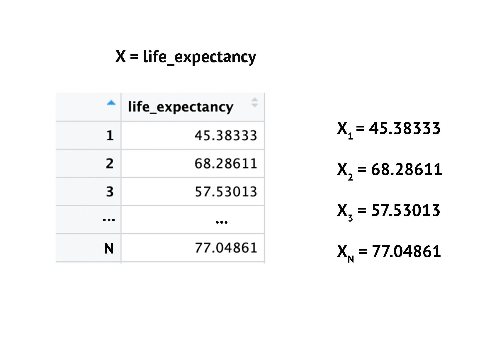
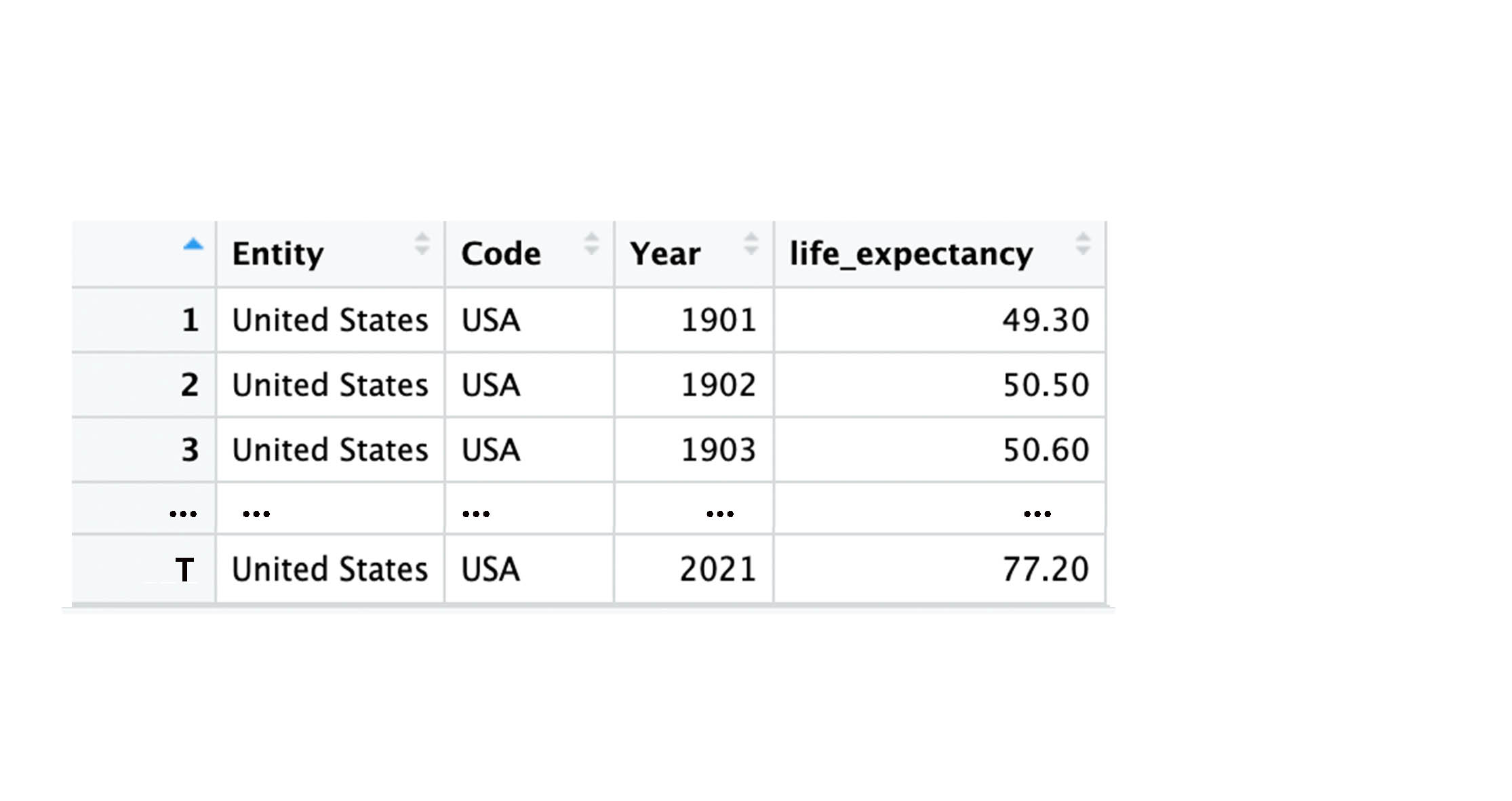
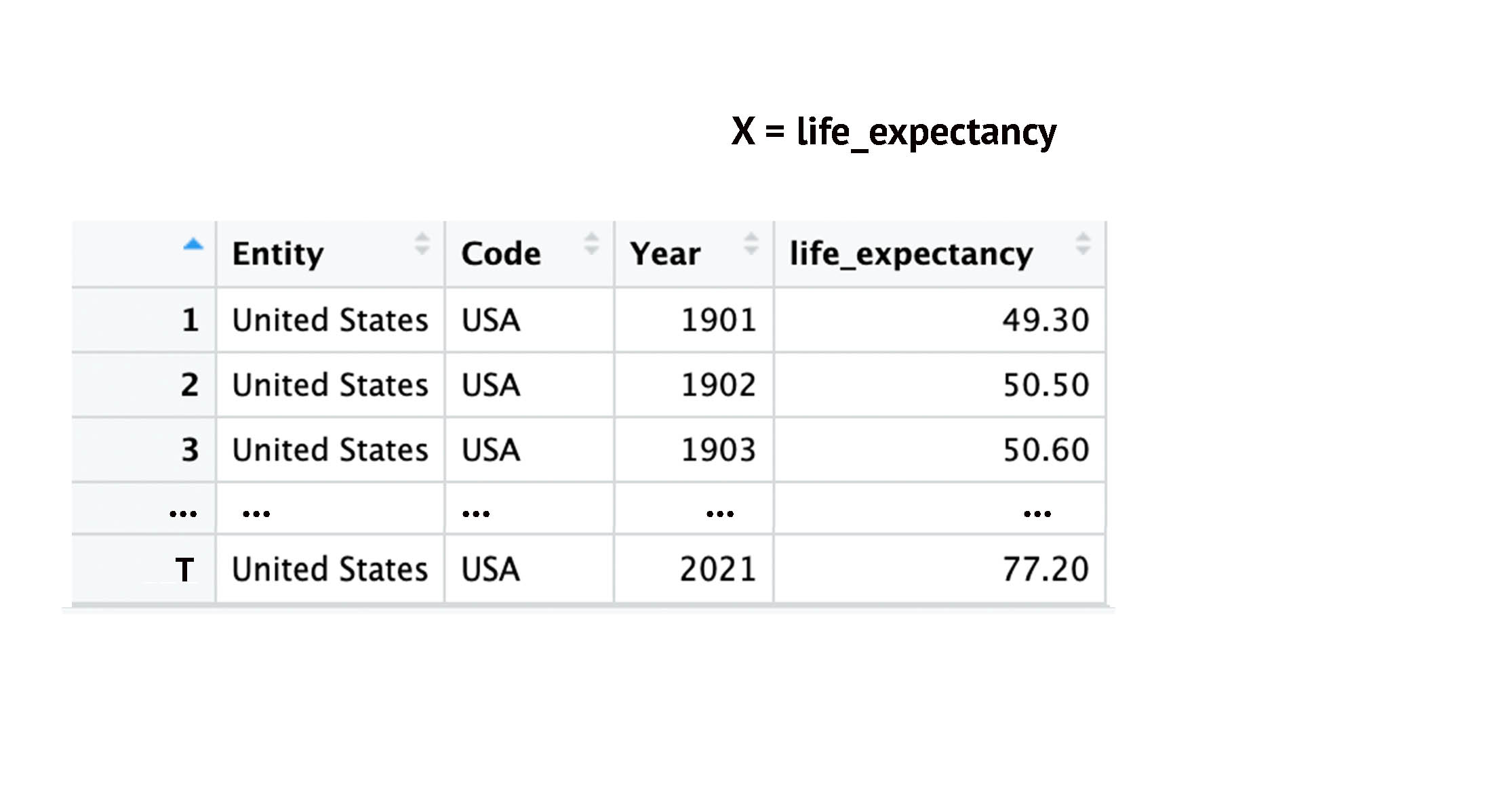
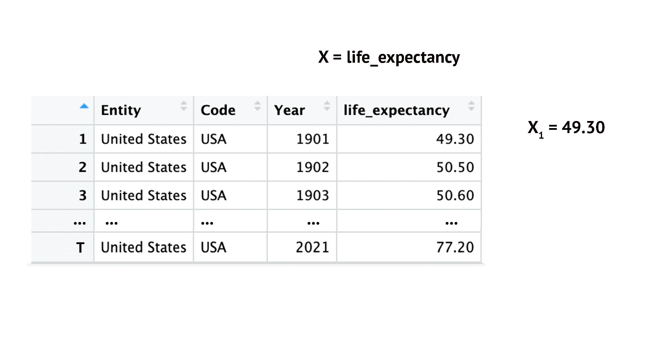
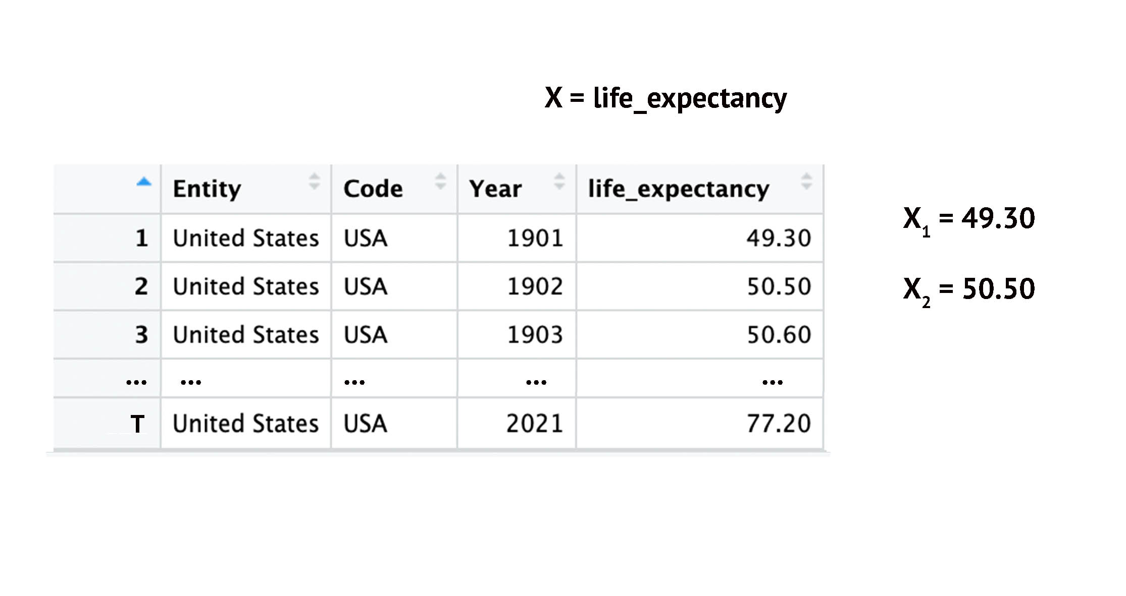
Cross-Sectional Data: Indexing
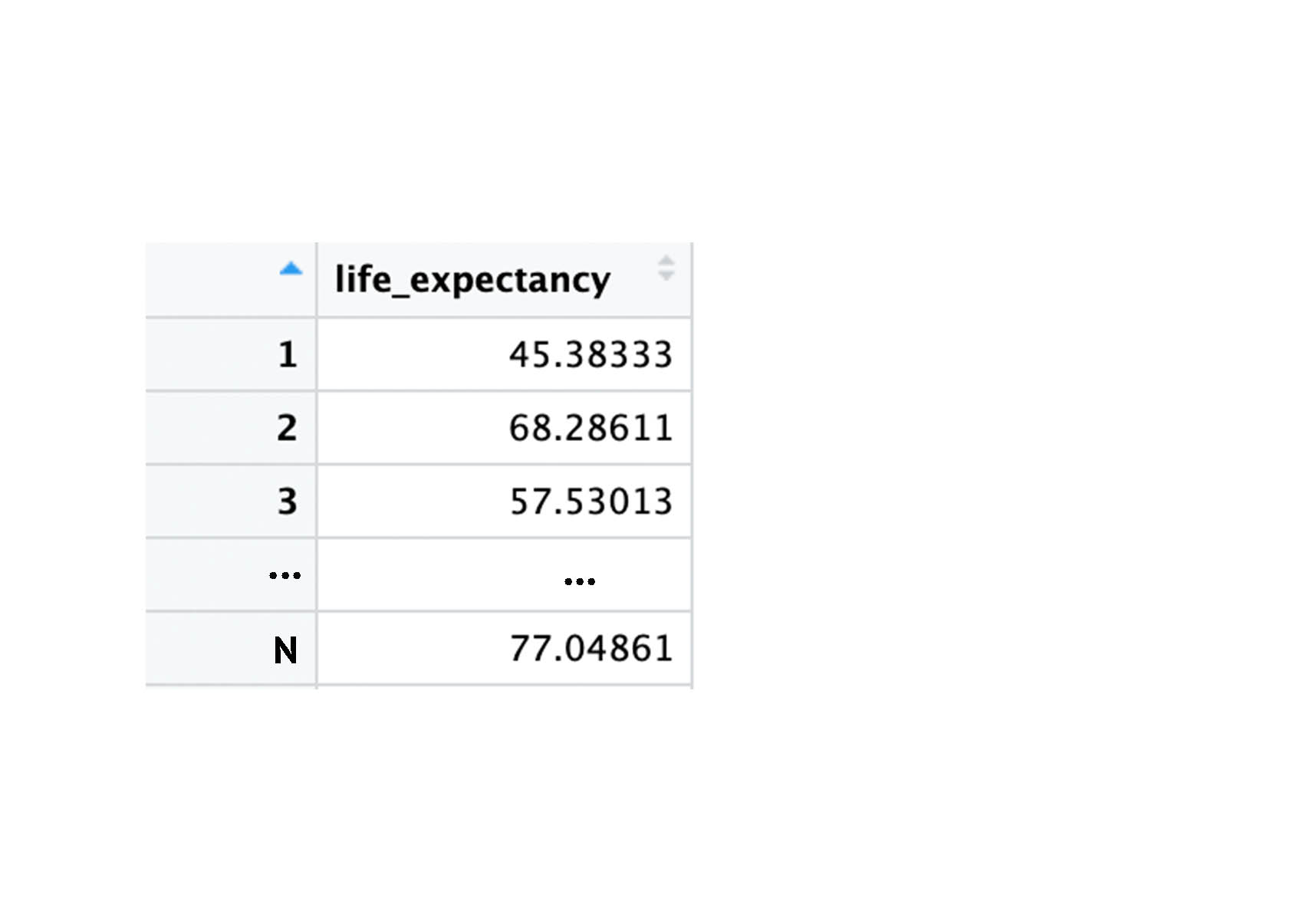
Cross-Sectional Data: Indexing
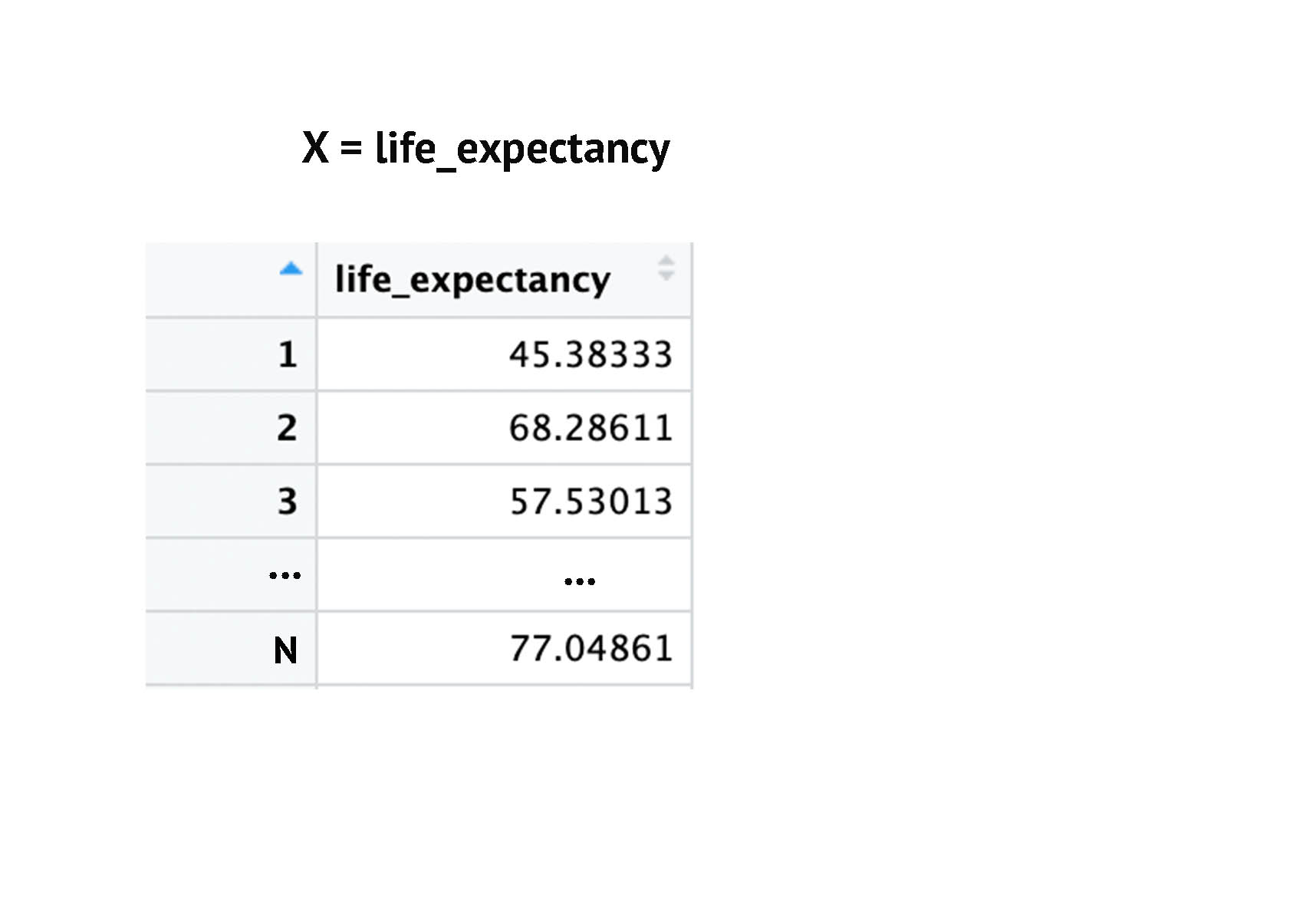
Cross-Sectional Data: Indexing
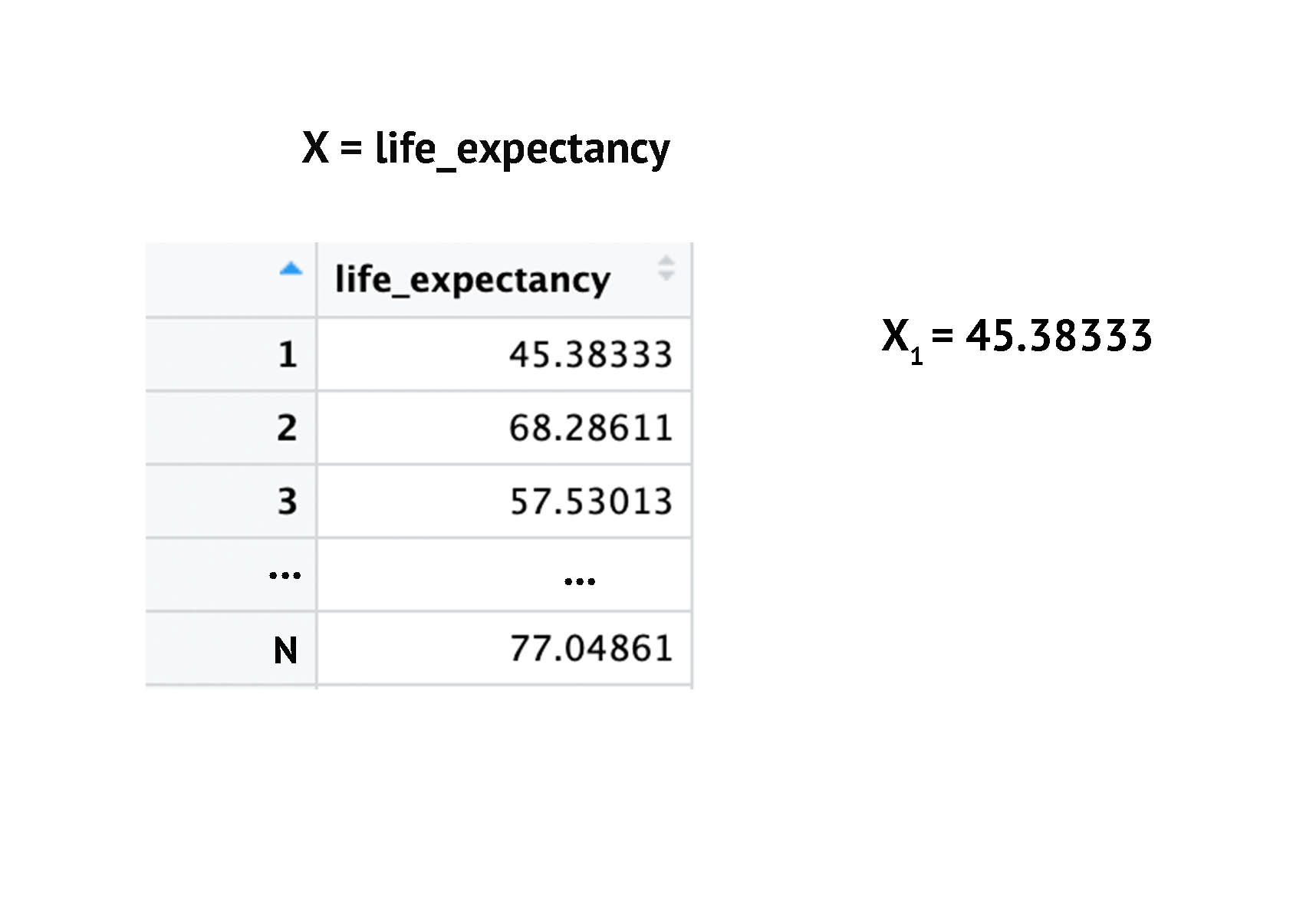
Cross-Sectional Data: Indexing
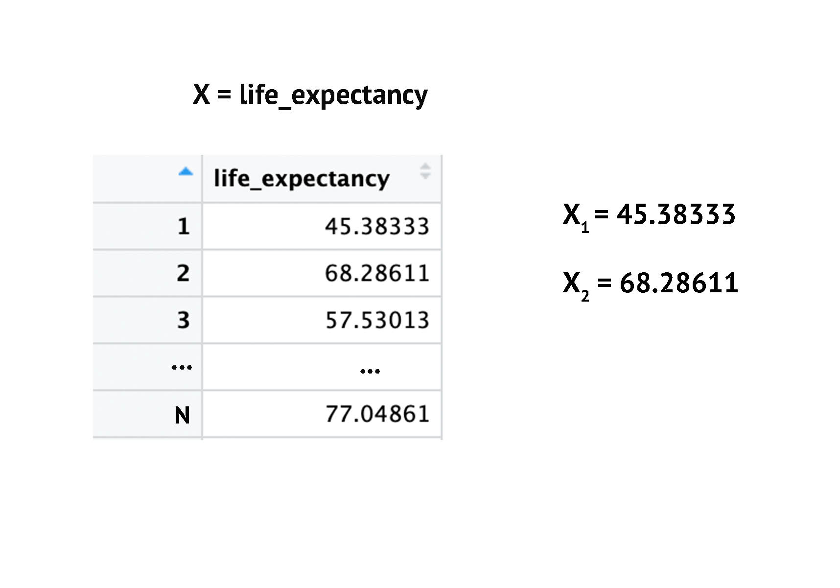
Cross-Sectional Data: Indexing
Scatterplot: One Country
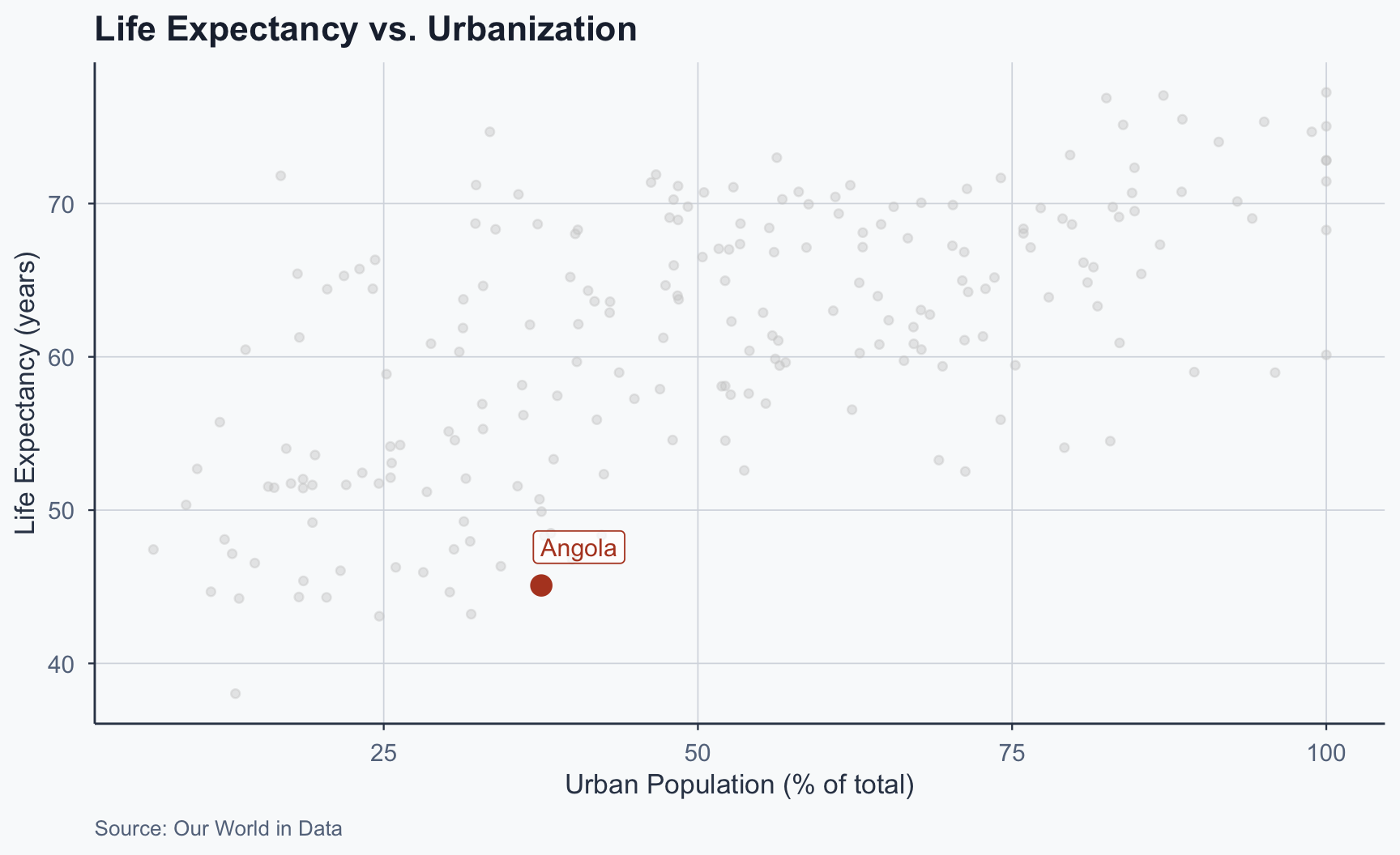
Figure 1
Scatterplot: Adding Countries
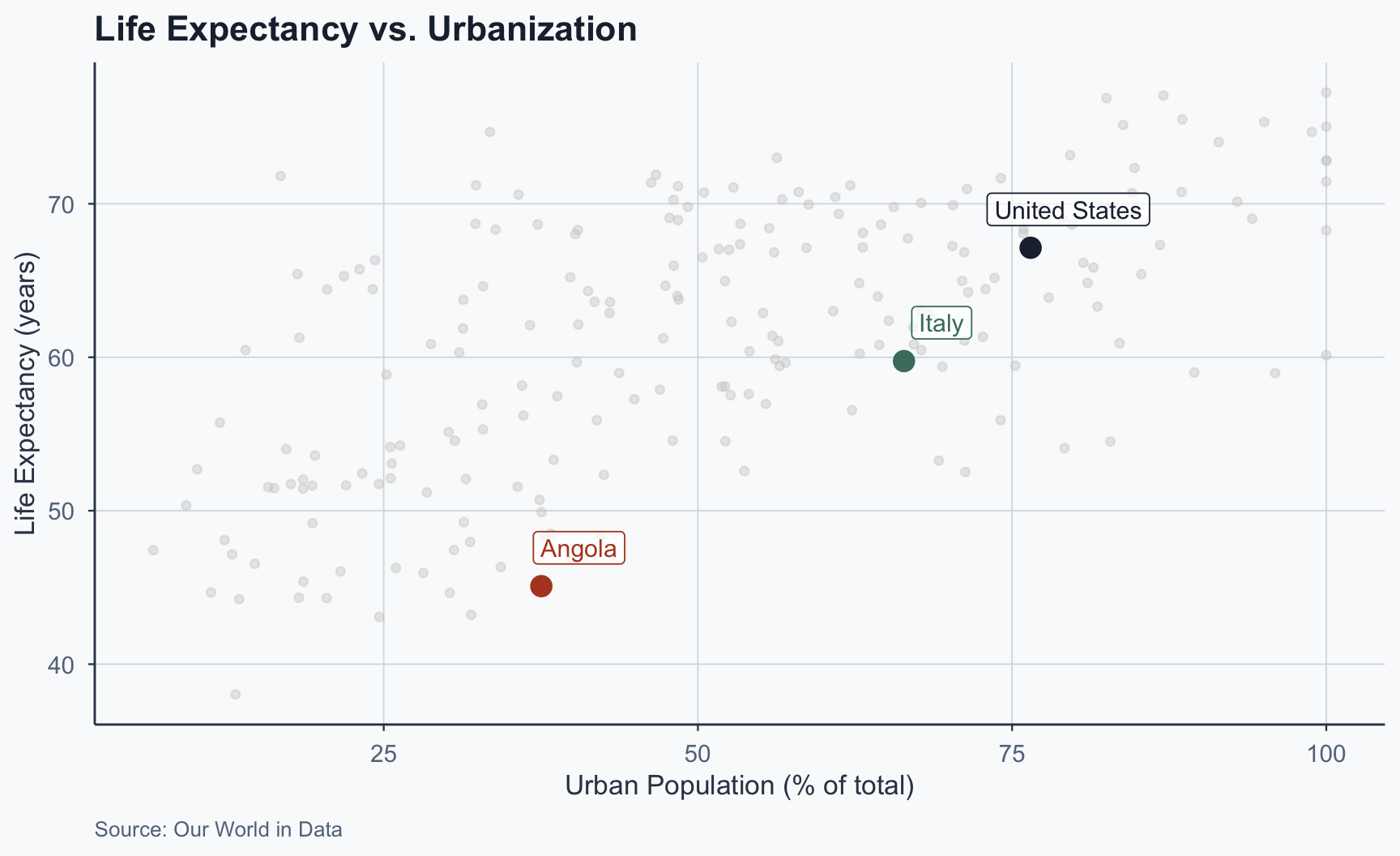
Figure 2
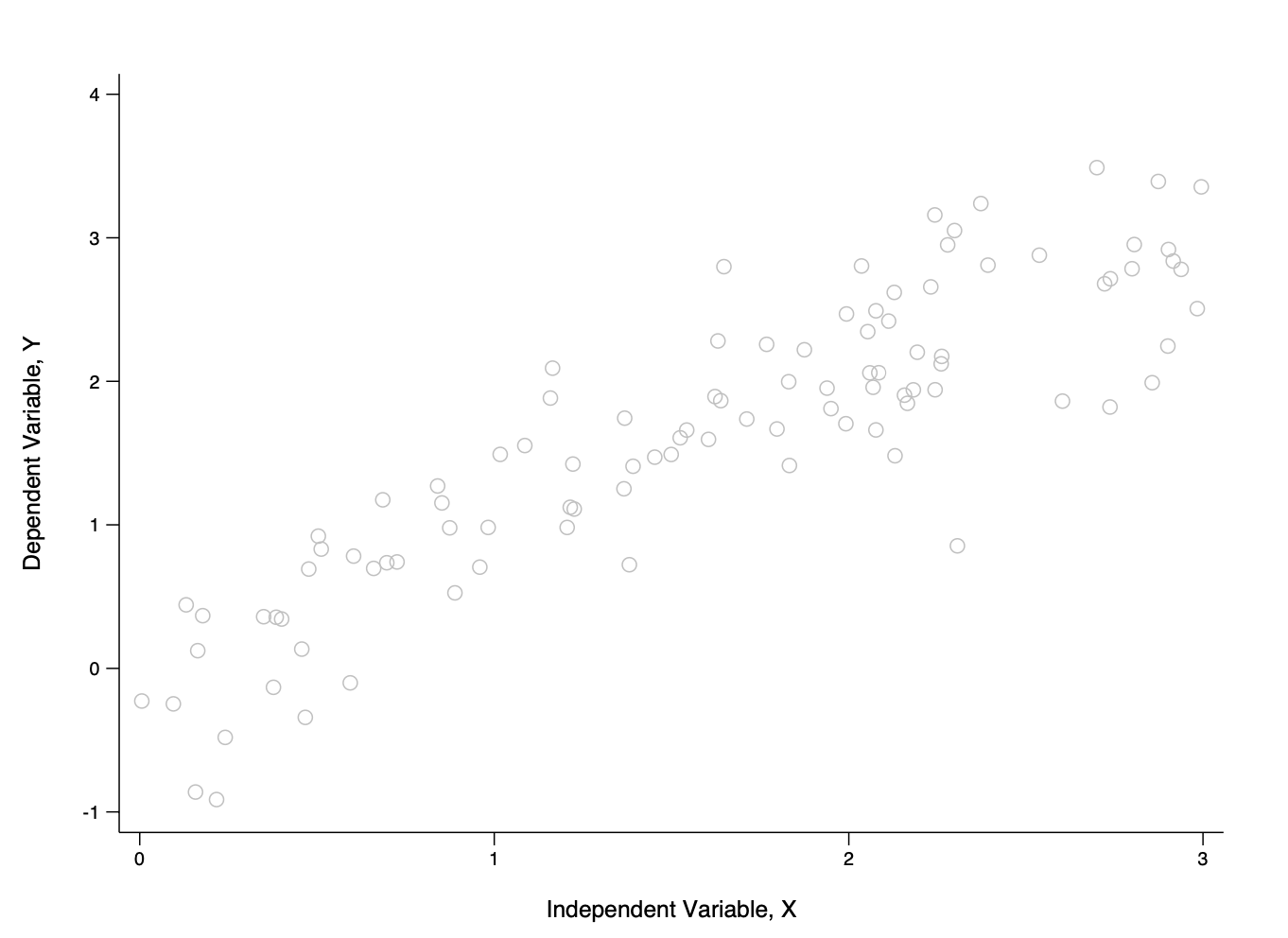
Scatterplot: All Countries
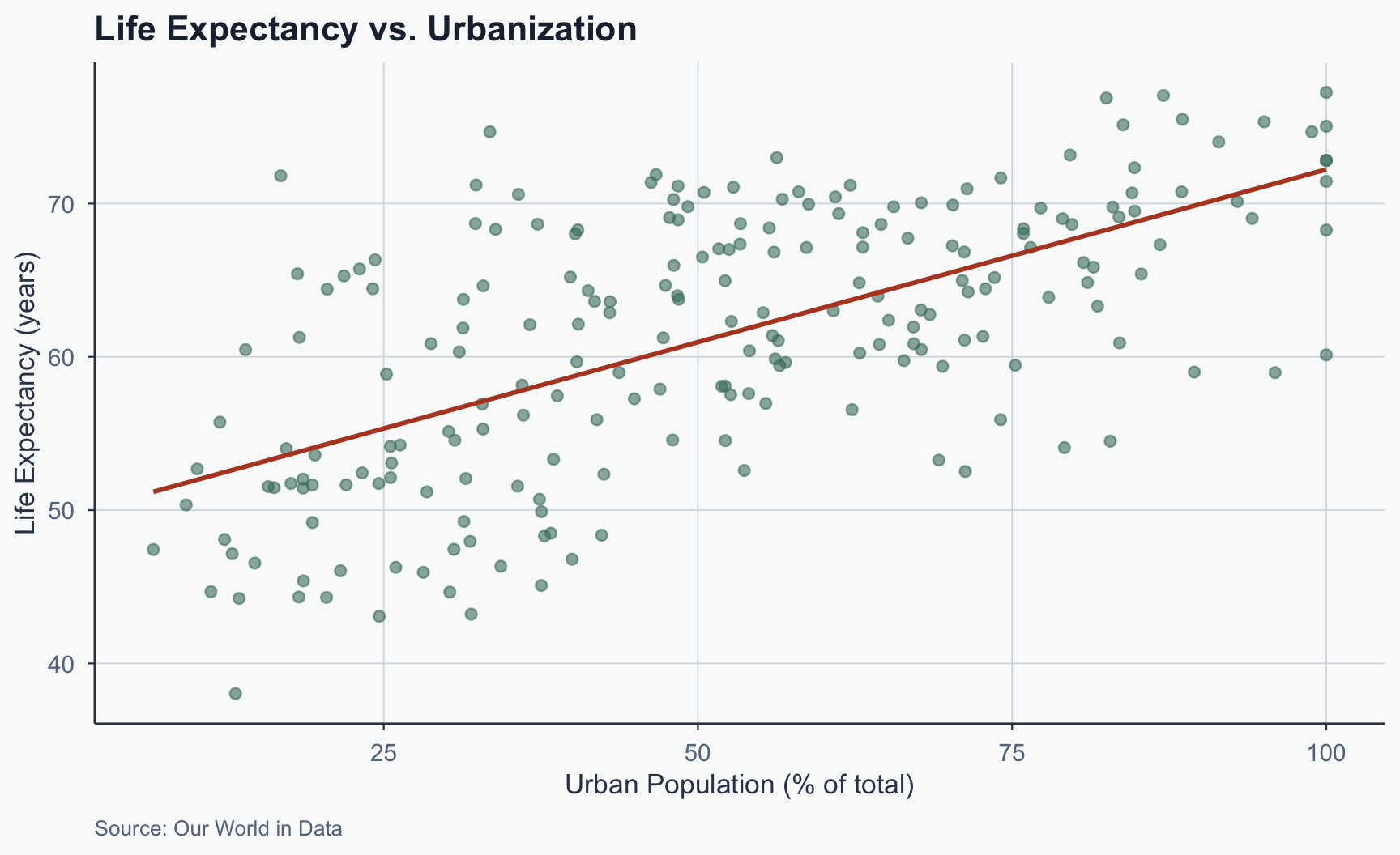
Figure 3
A Dataset
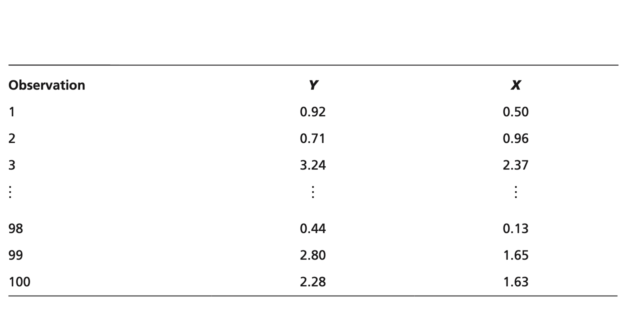
A Dataset: Variables Highlighted
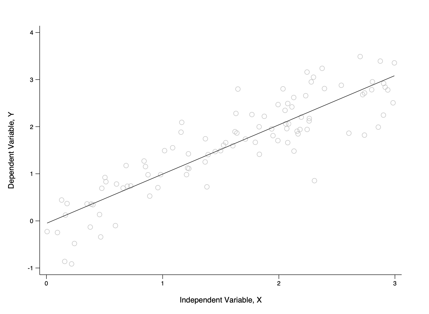
A Dataset: Trend Line
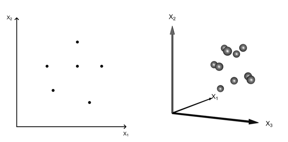
Three Dimensions
- Three variables \(\rightarrow\) 3D scatter cloud
- e.g., life expectancy, urbanization, education
Time-Series: Indexing
Time-Series: Indexing
Time-Series: Indexing
Time-Series: Indexing
Time-Series: Indexing
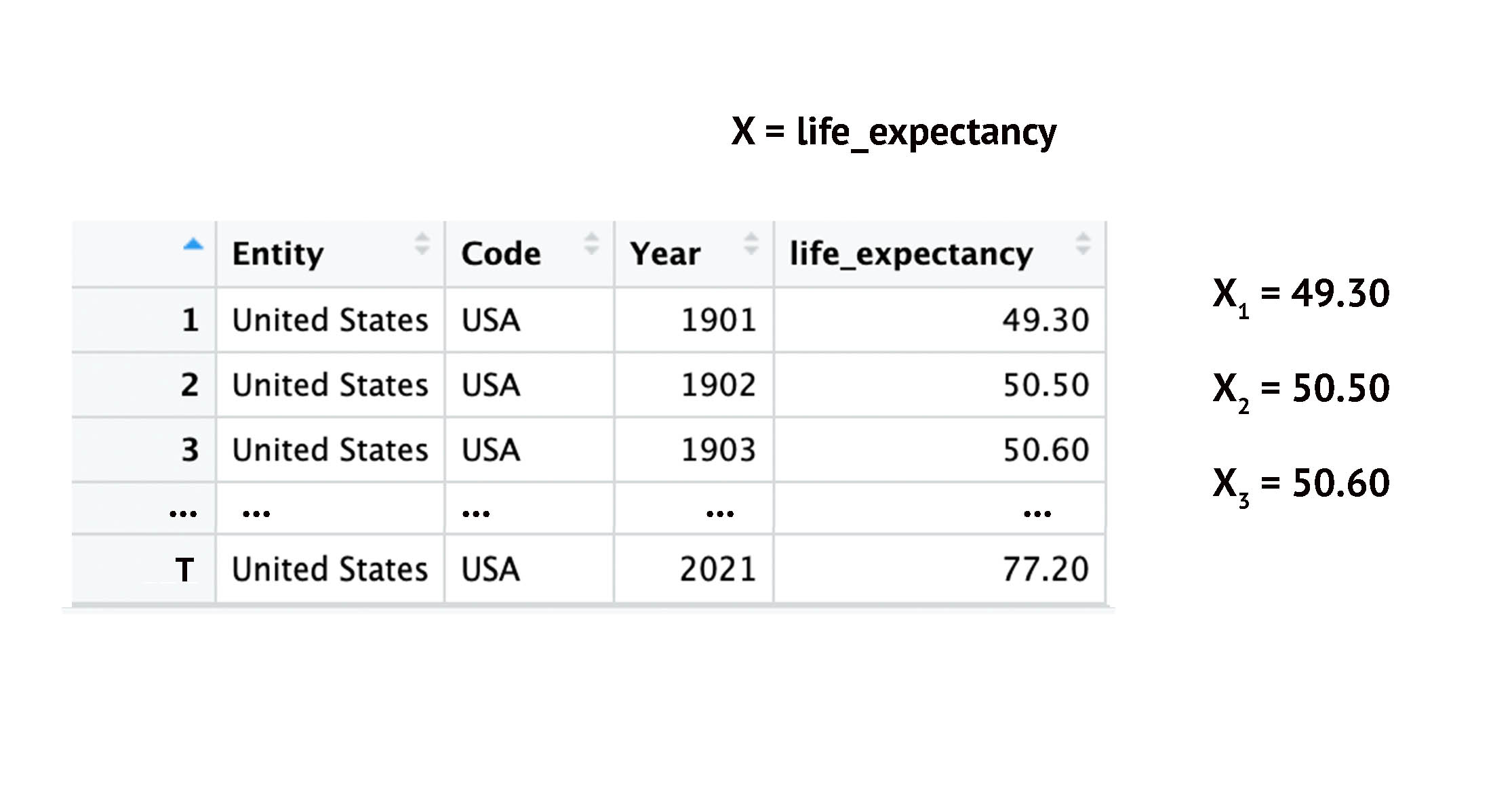
Time-Series: Indexing
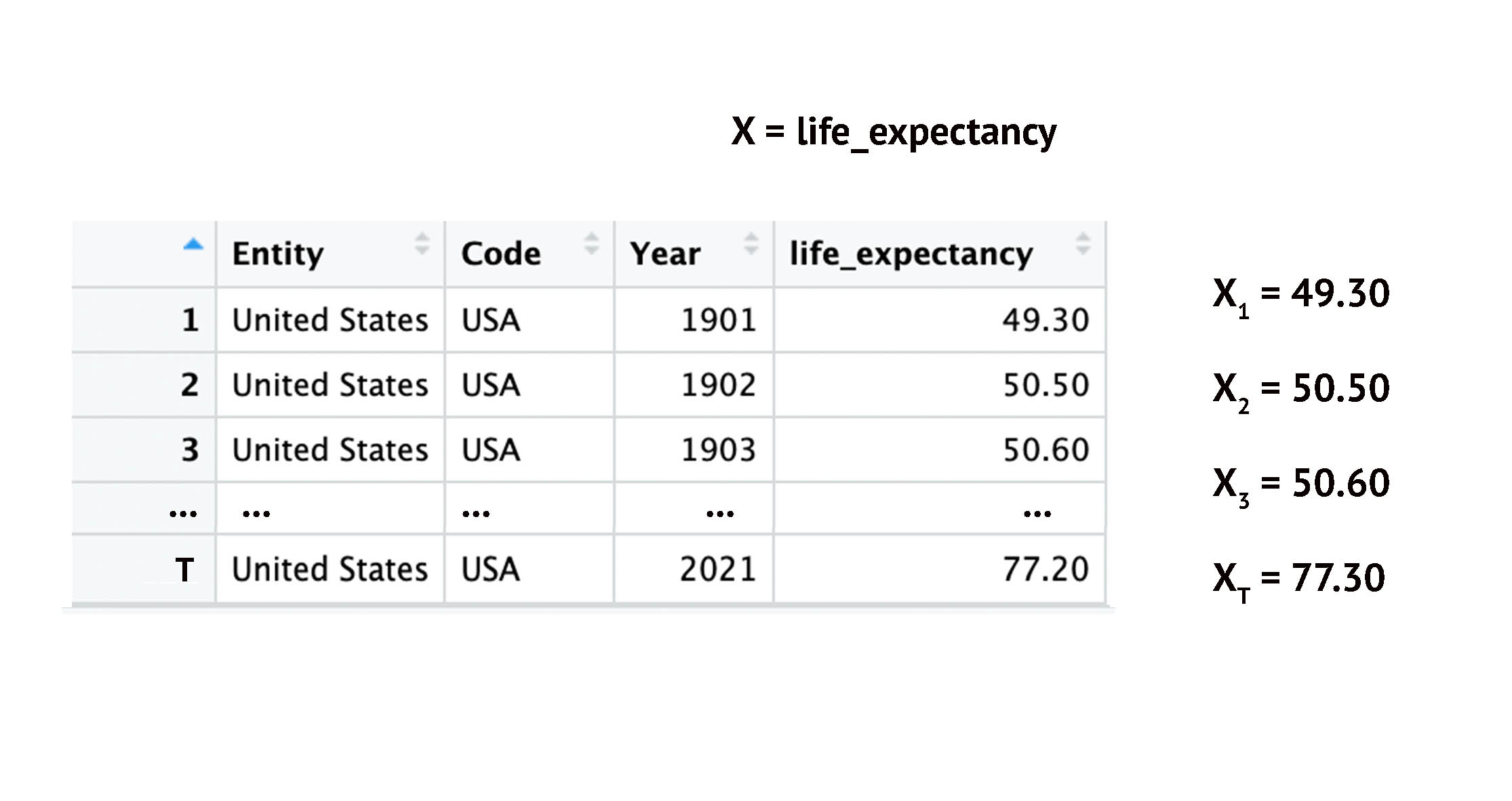
Time-Series: Indexing

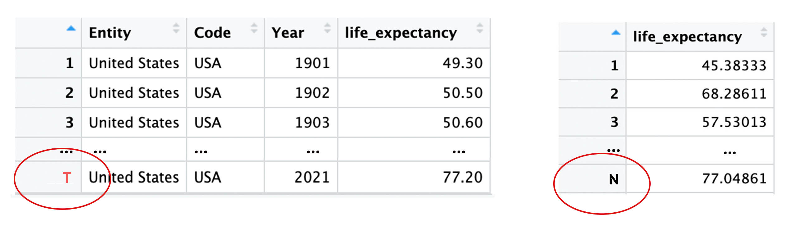
Time-Series vs. Cross-Section
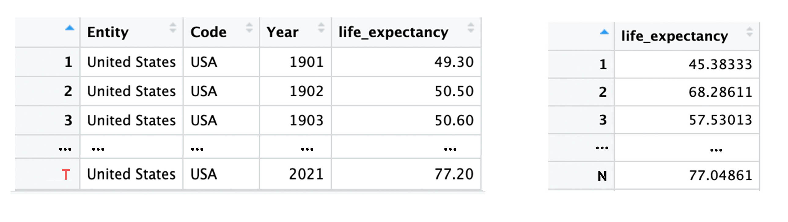
Time-Series vs. Cross-Section
USA: Life Expectancy Over Time
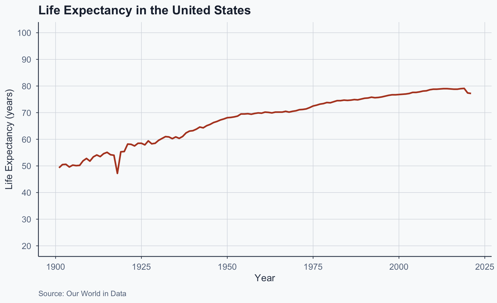
Figure 4
Panel Data: USA and Italy
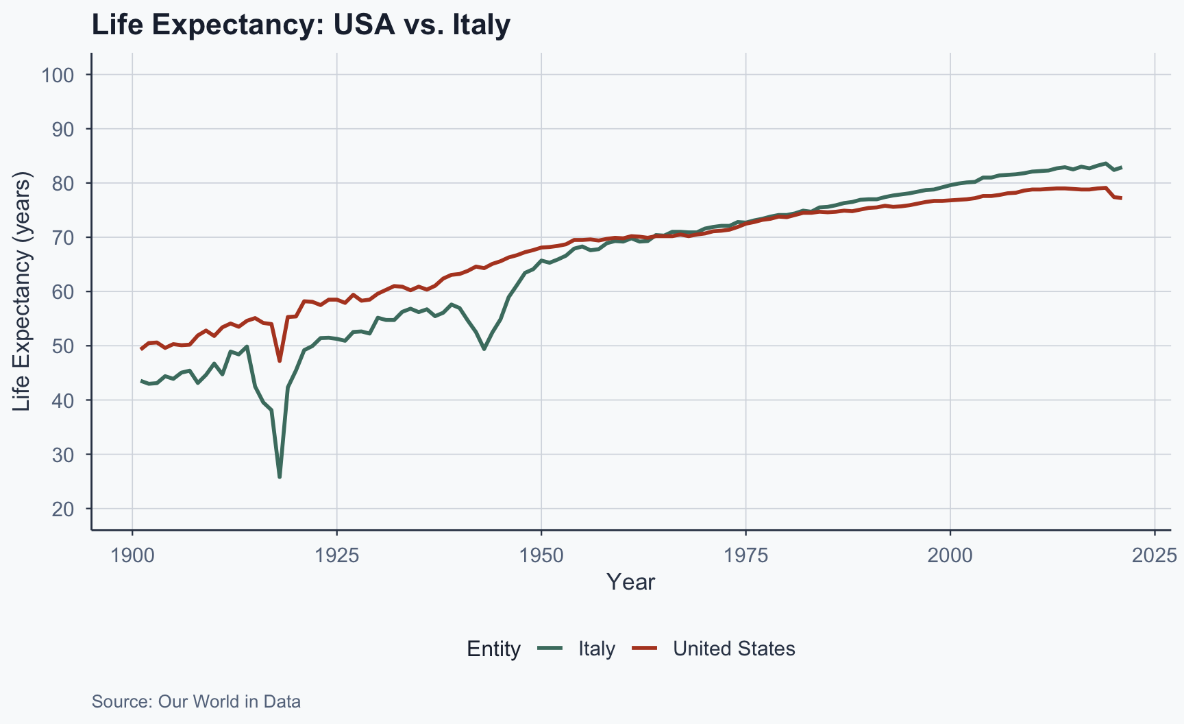
Figure 5
Balanced Panel: Three Countries
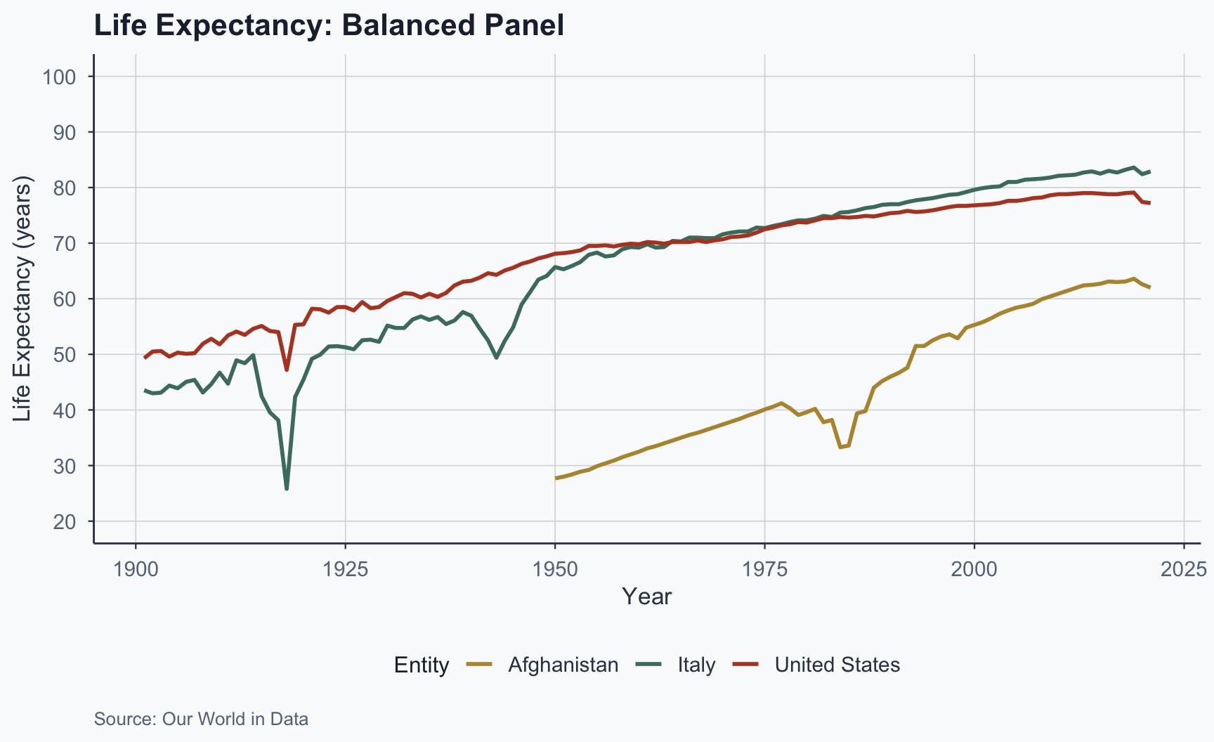
Figure 6
Unbalanced Panel: Four Countries
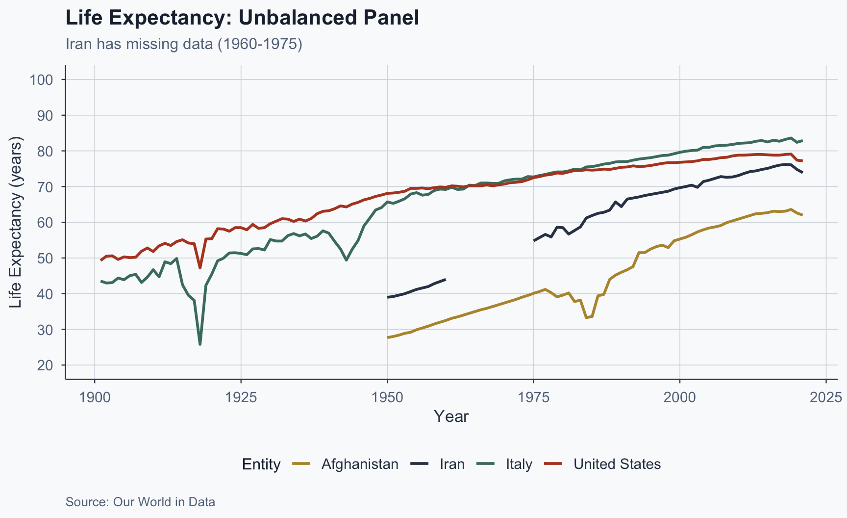
Figure 7