Statistical Analysis

Lecture 12: Threats to Validity

Bogdan G. Popescu

John Cabot University

Introduction

From Validity to Causal Inference

  • Previous week: DAGs, ATE, randomization
  • Today: threats to validity and how to address them
  • Key topics:
    • Construct, statistical, internal, and external validity
    • Matching and inverse probability weighting
  • Goal: improve causal claims from observational data

Construct Validity

Construct Validity

How well do our measures capture the concepts we care about?

Example: social anxiety is multidimensional:

  • Psychological: intense fear and anxiety
  • Physiological: physical stress indicators
  • Behavioral: avoidance of social settings
  • We must operationalize abstract ideas into observable indicators

Statistical Conclusion Validity

Type I and Type II Errors

Type I error (false positive):

  • Finding a relationship when none exists
  • Rejecting a true \(H_0\)

Type II error (false negative):

  • Missing a relationship that does exist
  • Failing to reject a false \(H_0\)

Statistical Power

Power = probability of detecting a true effect

When power is low:

  • Detecting true effects becomes difficult
  • Significant results less likely to reflect truth
  • Often caused by small sample sizes

p-Hacking

p-hacking: manipulating analyses to obtain significance

Common forms:

  1. Report only results that support the hypothesis
  2. Try multiple tests until one is significant
  3. Remove outliers to achieve desired results
  4. Not reporting null results

Threats to Internal Validity

Eight Threats to Internal Validity

# Threat Description
1 History External events affect results
2 Maturation Natural changes over time
3 Selection Bias Non-random group assignment
4 Attrition Dropout biases the sample
5 Regression to Mean Extremes moderate naturally
6 Hawthorne Effect Observation changes behavior
7 Placebo Effect Belief drives improvement
8 Spillover Treatment leaks to control group

History & Maturation

History: unrelated events during the study affect outcomes

  • A news event distracts students mid-experiment
  • Solution: use a control group

Maturation: participants change naturally over time

  • Children grow regardless of nutrition program
  • Solution: use a comparison group to remove trend

Selection Bias & Attrition

Selection bias: participants differ systematically from population

  • Volunteers are healthier than non-volunteers
  • Solution: randomization

Attrition: non-random dropout biases results

  • Patients not responding well leave the study
  • Solution: compare characteristics of stayers vs. leavers

Regression to Mean & Hawthorne

Regression to mean: extreme values moderate naturally

  • Very overweight participants lose some weight naturally
  • Solution: don’t select extremes

Hawthorne effect: behavior changes under observation

  • Workers are more productive when being watched
  • Solution: use a control group also under observation

Placebo & Spillover

Placebo effect: belief in treatment causes improvement

  • Control group improves from receiving inert treatment
  • Solution: include a placebo group (double-blind)

Spillover: treatment leaks to control group

  • Treated students share knowledge with untreated peers
  • Solution: use geographically distant control groups

Hawthorne vs. Placebo

These are commonly confused:

  • Hawthorne: behavior changes from being observed
    • Participants know they are in a study
  • Placebo: improvement from believing in treatment
    • Participants are unaware they receive no active treatment

What Randomization Fixes

Randomization addresses some but not all threats:

  • Fixes: selection bias, maturation, regression to mean
  • Does not fix: attrition, spillover, measurement problems
  • Additional safeguards are always needed

Threats to External Validity

External Validity

Are your findings generalizable to the whole population?

  • Many study participants are WEIRD:
    • Western, Educated, Industrialized, Rich, Democratic
  • We must assess how findings extend to other populations

Sample Selection & Contextual Factors

Sample selection: the sample does not represent the population

  • Drug study selects only ages 20–30
  • Solution: select representative samples

Contextual factors: setting influences results

  • Counseling program works at one university but not others
  • Solution: replicate across multiple settings

Types of Research

Experimental Studies

  • Researcher manipulates the independent variable
  • Participants randomly assigned to groups
  • Stronger claims about cause and effect
  • More expensive and time-consuming

Observational Studies

  • Researcher observes without manipulating
  • Participants are not randomly assigned
  • Useful for real-world behaviors and outcomes
  • More prone to bias and confounding

Improving Observational Studies

Four techniques to approach causal estimates:

  1. Matching: pair similar treated/untreated units
  2. Instrumental variables: use an exogenous instrument
  3. Regression discontinuity: compare at a threshold
  4. Difference-in-differences: compare changes over time

Today: matching and inverse probability weighting

Nearest Neighbor Matching

What Is Matching?

Matching: create comparable groups by pairing similar units

  • Reduces bias from confounding variables
  • Pairs treated and untreated on pre-treatment characteristics
  • Goal: make groups comparable as if randomized

The Malaria Example

Back to the malaria study — now observational:

  • People choose to use nets
  • No random assignment
  • Confounders affect treatment
Show Code
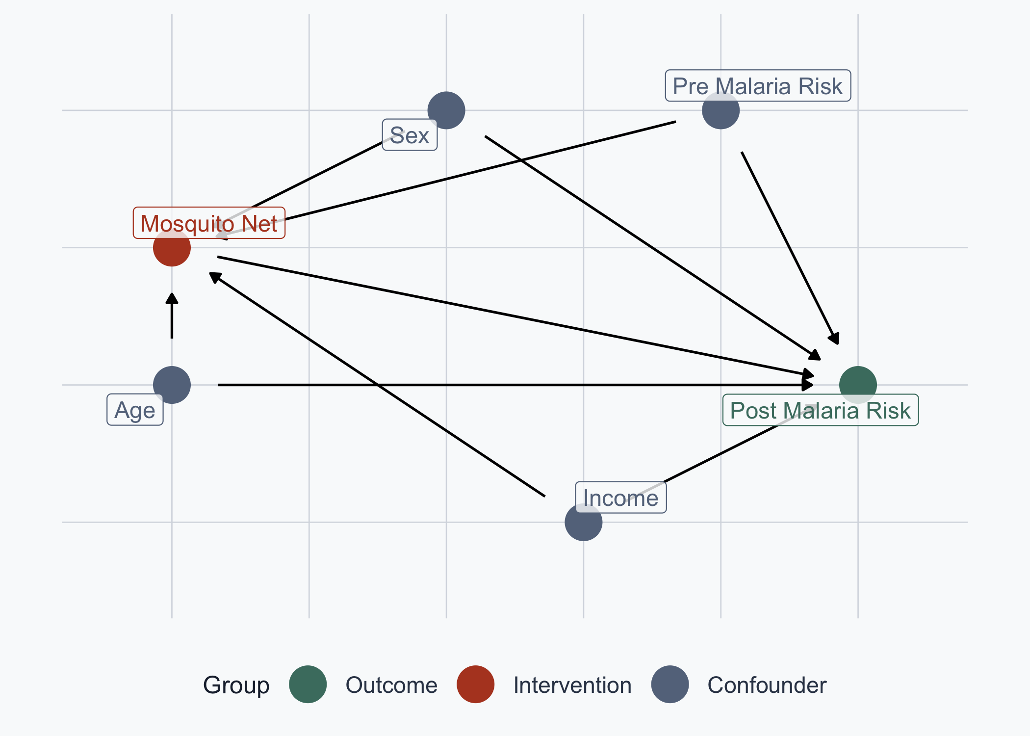
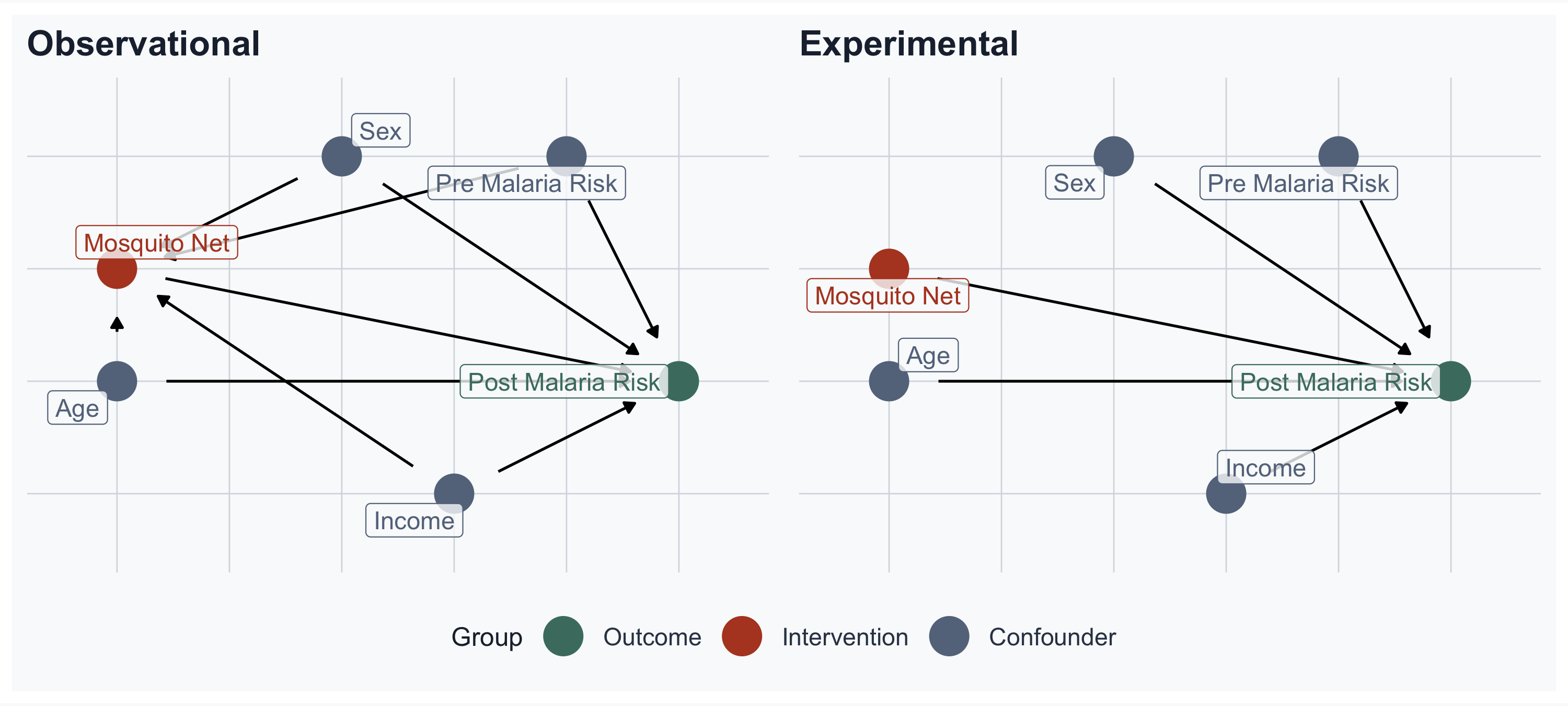
# Observational DAG: confounders -> Net AND -> Post Malaria Risk
malaria_dag_obs <- dagify(
  post_malaria_risk ~ net + age + sex + income + pre_malaria_risk,
  net ~ age + sex + income + pre_malaria_risk,
  exposure = "net",
  outcome = "post_malaria_risk",
  labels = c(post_malaria_risk = "Post Malaria Risk",
             net = "Mosquito Net",
             age = "Age", sex = "Sex",
             income = "Income",
             pre_malaria_risk = "Pre Malaria Risk"),
  coords = list(
    x = c(net = 2, post_malaria_risk = 7, income = 5,
          age = 2, sex = 4, pre_malaria_risk = 6),
    y = c(net = 3, post_malaria_risk = 2, income = 1,
          age = 2, sex = 4, pre_malaria_risk = 4)
  )
)

# Cleaning the DAG and turning it into a dataframe
df_obs <- data.frame(tidy_dagitty(malaria_dag_obs))
df_obs$type <- "Confounder"
df_obs$type[df_obs$name == "post_malaria_risk"] <- "Outcome"
df_obs$type[df_obs$name == "net"] <- "Intervention"

# Axis limits
min_lon_x <- min(df_obs$x, na.rm = TRUE)
max_lon_x <- max(df_obs$x, na.rm = TRUE)
min_lat_y <- min(df_obs$y, na.rm = TRUE)
max_lat_y <- max(df_obs$y, na.rm = TRUE)
error <- (max_lon_x - min_lon_x) / 10

# Producing the graph
dag_obs_plot <- ggplot(df_obs,
    aes(x = x, y = y, xend = xend, yend = yend, color = type)) +
  geom_dag_point(size = 8) +
  geom_dag_edges() +
  scale_colour_manual(values = dag_col, name = "Group",
                      breaks = dag_order) +
  geom_label_repel(
    data = subset(df_obs, !duplicated(df_obs$label)),
    aes(label = label),
    fill = alpha(cream, 0.8), size = 4,
    show.legend = FALSE) +
  coord_sf(xlim = c(min_lon_x - error, max_lon_x + error),
           ylim = c(min_lat_y - error, max_lat_y + error)) +
  labs(x = NULL, y = NULL) +
  theme_meridian() +
  theme(axis.text = element_blank(),
        axis.line = element_blank(),
        axis.ticks = element_blank(),
        panel.grid = element_blank())

dag_obs_plot

Observational vs. Experimental

Show Code
# Experimental DAG: confounders -> Post Malaria Risk only (no arrows into Net)
malaria_dag_exp <- dagify(
  post_malaria_risk ~ net + age + sex + income + pre_malaria_risk,
  exposure = "net",
  outcome = "post_malaria_risk",
  labels = c(post_malaria_risk = "Post Malaria Risk",
             net = "Mosquito Net",
             age = "Age", sex = "Sex",
             income = "Income",
             pre_malaria_risk = "Pre Malaria Risk"),
  coords = list(
    x = c(net = 2, post_malaria_risk = 7, income = 5,
          age = 2, sex = 4, pre_malaria_risk = 6),
    y = c(net = 3, post_malaria_risk = 2, income = 1,
          age = 2, sex = 4, pre_malaria_risk = 4)
  )
)

# Cleaning the DAG and turning it into a dataframe
df_exp <- data.frame(tidy_dagitty(malaria_dag_exp))
df_exp$type <- "Confounder"
df_exp$type[df_exp$name == "post_malaria_risk"] <- "Outcome"
df_exp$type[df_exp$name == "net"] <- "Intervention"

# Producing the graph
dag_exp_plot <- ggplot(df_exp,
    aes(x = x, y = y, xend = xend, yend = yend, color = type)) +
  geom_dag_point(size = 8) +
  geom_dag_edges() +
  scale_colour_manual(values = dag_col, name = "Group",
                      breaks = dag_order) +
  geom_label_repel(
    data = subset(df_exp, !duplicated(df_exp$label)),
    aes(label = label),
    fill = alpha(cream, 0.8), size = 4,
    show.legend = FALSE) +
  coord_sf(xlim = c(min_lon_x - error, max_lon_x + error),
           ylim = c(min_lat_y - error, max_lat_y + error)) +
  labs(x = NULL, y = NULL) +
  theme_meridian() +
  theme(axis.text = element_blank(),
        axis.line = element_blank(),
        axis.ticks = element_blank(),
        panel.grid = element_blank())

# Side-by-side comparison
(dag_obs_plot + ggtitle("Observational")) +
  (dag_exp_plot + ggtitle("Experimental")) +
  plot_layout(guides = "collect") &
  theme(legend.position = "bottom")

The Model

\[\text{Malaria Risk} = \beta_0 + \beta_1 \cdot \text{Net} + \beta_2 \cdot \text{Income} + \epsilon\]

Show Code
mod_naive <- lm(malaria_risk_post ~ net, data = rct)
b_naive <- round(coef(mod_naive)["net"], 3)

ggplot(rct, aes(x = income, y = malaria_risk_post,
                color = type, shape = type)) +
  geom_point(alpha = 0.5, size = 1.5) +
  geom_smooth(method = "lm", se = FALSE, linewidth = 0.8) +
  scale_color_manual(values = c("Control" = stone, "Treatment" = terracotta)) +
  scale_shape_manual(values = c(16, 17)) +
  labs(title = "Malaria Risk vs. Income by Treatment",
       x = "Income", y = "Post-Treatment Malaria Risk",
       color = "", shape = "",
       caption = "Source: Simulated Malawi RCT data") +
  theme_meridian()

Naive Estimate

mod_naive <- lm(malaria_risk_post ~ net, data = rct)
summary(mod_naive)

Call:
lm(formula = malaria_risk_post ~ net, data = rct)

Residuals:
     Min       1Q   Median       3Q      Max 
-30.5794  -6.4719   0.0798   6.1909  28.9747 

Coefficients:
            Estimate Std. Error t value Pr(>|t|)    
(Intercept)  45.6621     0.4146  110.14   <2e-16 ***
net         -10.0827     0.5738  -17.57   <2e-16 ***
---
Signif. codes:  0 '***' 0.001 '**' 0.01 '*' 0.05 '.' 0.1 ' ' 1

Residual standard error: 9.064 on 998 degrees of freedom
Multiple R-squared:  0.2363,    Adjusted R-squared:  0.2355 
F-statistic: 308.7 on 1 and 998 DF,  p-value: < 2.2e-16

Confounders Drive Treatment

Higher income and higher pre-malaria risk \(\rightarrow\) more likely to use nets

Show Code
ggplot(rct, aes(x = income, y = malaria_risk_pre,
                color = type, shape = type)) +
  geom_point(alpha = 0.5, size = 1.5) +
  scale_color_manual(values = c("Control" = stone, "Treatment" = terracotta)) +
  scale_shape_manual(values = c(16, 17)) +
  labs(title = "Pre-Treatment Confounders by Group",
       x = "Income", y = "Pre-Treatment Malaria Risk",
       color = "", shape = "",
       caption = "Source: Simulated Malawi RCT data") +
  theme_meridian()

Process for Matching

Step 1: identify confounders from the DAG

  • Income and pre-malaria risk affect net usage

Step 2: match treated and untreated on confounders

  • Find similar pairs who differ only in treatment

Step 3: estimate treatment effect on matched data

Nearest Neighbor Matching in R

matched_ob <- matchit(net ~ income + malaria_risk_pre,
                       data = rct, method = "nearest",
                       distance = "mahalanobis",
                       replace = FALSE)
matched_ob
A `matchit` object
 - method: 1:1 nearest neighbor matching without replacement
 - distance: Mahalanobis - number of obs.: 1000 (original), 956 (matched)
 - target estimand: ATT
 - covariates: income, malaria_risk_pre

Before vs. After Matching

Show Code
rct$source <- "All Data"
matched$source <- "Matched"

p_before <- ggplot(rct, aes(x = income, y = malaria_risk_pre,
                             color = type, shape = type)) +
  geom_point(alpha = 0.4, size = 1.3) +
  scale_color_manual(values = c("Control" = stone, "Treatment" = terracotta)) +
  scale_shape_manual(values = c(16, 17)) +
  labs(title = "Before Matching",
       x = "Income", y = "Pre-Malaria Risk",
       color = "", shape = "") +
  theme_meridian(base_size = 11)

matched$type <- ifelse(matched$net == 1, "Treatment", "Control")

p_after <- ggplot(matched, aes(x = income, y = malaria_risk_pre,
                                color = type, shape = type)) +
  geom_point(alpha = 0.5, size = 1.3) +
  scale_color_manual(values = c("Control" = stone, "Treatment" = terracotta)) +
  scale_shape_manual(values = c(16, 17)) +
  labs(title = "After Matching",
       x = "Income", y = "Pre-Malaria Risk",
       color = "", shape = "") +
  theme_meridian(base_size = 11)

p_before + p_after +
  plot_annotation(caption = "Source: Simulated Malawi RCT data")

Matched vs. Unmatched Results

mod_matched <- lm(malaria_risk_post ~ net, data = matched)
summary(mod_matched)

Call:
lm(formula = malaria_risk_post ~ net, data = matched)

Residuals:
     Min       1Q   Median       3Q      Max 
-30.5936  -6.5821   0.0878   6.3101  28.9605 

Coefficients:
            Estimate Std. Error t value Pr(>|t|)    
(Intercept)  45.6621     0.4168  109.55   <2e-16 ***
net         -10.0685     0.5895  -17.08   <2e-16 ***
---
Signif. codes:  0 '***' 0.001 '**' 0.01 '*' 0.05 '.' 0.1 ' ' 1

Residual standard error: 9.113 on 954 degrees of freedom
Multiple R-squared:  0.2342,    Adjusted R-squared:  0.2334 
F-statistic: 291.8 on 1 and 954 DF,  p-value: < 2.2e-16

Drawbacks of NN Matching

  • One-to-one matching drops many observations
  • Original: 1000 \(\rightarrow\) Matched: 956
  • Smaller samples reduce statistical power
  • Results may be sensitive to matching specification
  • Alternative: Inverse Probability Weighting keeps all data

Inverse Probability Weighting

What Is IPW?

Inverse Probability Weighting: reweight observations instead of dropping them

  • Predict the probability of treatment (propensity score)
  • Give more weight to “surprising” observations
  • Keep all data \(\rightarrow\) no loss of sample size

Logistic Regression

To compute propensity scores, we use logistic regression:

\[\log\frac{P(\text{Treated})}{1 - P(\text{Treated})} = \beta_0 + \beta_1 X_1 + \beta_2 X_2\]

  • Predicts the probability of receiving treatment
  • Output is bounded between 0 and 1 (S-curve)

Logistic Regression: mtcars Example

Show Code
ggplot(mtcars, aes(x = mpg, y = am)) +
  geom_point(color = sage, alpha = 0.6, size = 2) +
  stat_smooth(method = "glm",
              method.args = list(family = "binomial"),
              se = TRUE, color = terracotta, linewidth = 1) +
  labs(title = "Logistic Regression: Manual Transmission vs. MPG",
       x = "Miles per Gallon", y = "Prob. of Manual Transmission",
       caption = "Source: mtcars dataset") +
  theme_meridian()

Interpreting Odds Ratios

model_car <- glm(am ~ mpg, data = mtcars,
                 family = binomial(link = "logit"))
tidy(model_car, exponentiate = TRUE)
# A tibble: 2 × 5
  term        estimate std.error statistic p.value
  <chr>          <dbl>     <dbl>     <dbl>   <dbl>
1 (Intercept)  0.00136     2.35      -2.81 0.00498
2 mpg          1.36        0.115      2.67 0.00751
  • Odds ratio centered around 1 (no effect)
  • OR \(> 1\): more likely (e.g., 1.36 = 36% more likely)
  • OR \(< 1\): less likely (subtract from 1)

The Weighting Idea

Make underrepresented groups count more:

Group Population Sample Weight
Young 30% 60% 30/60 = 0.5
Middle 40% 30% 40/30 = 1.33
Old 30% 10% 30/10 = 3.0
  • Old people are upweighted (underrepresented)
  • Young people are downweighted (overrepresented)

IPW Formula

\[w_i = \frac{T_i}{p_i} + \frac{1 - T_i}{1 - p_i}\]

where \(T_i\) = treatment status, \(p_i\) = propensity score

  • High propensity + no treatment \(\rightarrow\) high weight
  • Low propensity + treatment \(\rightarrow\) high weight
  • “Surprising” observations get more influence

IPW Applied to Malaria

Show Code
# Step 1: Logistic regression for propensity
model_prop <- glm(net ~ income + malaria_risk_pre,
                  data = rct,
                  family = binomial(link = "logit"))

# Step 2: Get propensity scores
rct_ipw <- rct
rct_ipw$propensity <- predict(model_prop, type = "response")

# Step 3: Compute IPW weights
rct_ipw$ipw <- rct_ipw$net / rct_ipw$propensity +
               (1 - rct_ipw$net) / (1 - rct_ipw$propensity)
Show Code
p_unw <- ggplot(rct_ipw, aes(x = income, y = malaria_risk_pre,
                               color = type, shape = type)) +
  geom_point(size = 1.5, alpha = 0.5) +
  scale_color_manual(values = c("Control" = stone, "Treatment" = terracotta)) +
  scale_shape_manual(values = c(16, 17)) +
  labs(title = "Unweighted", x = "Income", y = "Pre-Malaria Risk",
       color = "", shape = "") +
  theme_meridian(base_size = 11)

p_wt <- ggplot(rct_ipw, aes(x = income, y = malaria_risk_pre,
                              color = type, shape = type,
                              size = ipw)) +
  geom_point(alpha = 0.5) +
  scale_color_manual(values = c("Control" = stone, "Treatment" = terracotta)) +
  scale_shape_manual(values = c(16, 17)) +
  scale_size_continuous(range = c(0.5, 5), guide = "none") +
  labs(title = "IPW Weighted", x = "Income", y = "Pre-Malaria Risk",
       color = "", shape = "") +
  theme_meridian(base_size = 11)

p_unw + p_wt +
  plot_annotation(caption = "Source: Simulated Malawi RCT data")

Comparing Methods

Three Approaches Compared

Effect of mosquito nets on post-treatment malaria risk
Model Net Estimate Std. Error p-value N
Naive Regression -10.083 0.574 0 1000
NN Matched -10.069 0.589 0 956
IPW Weighted -10.075 0.572 0 1000
  • All three methods find a negative treatment effect
  • Matched and IPW adjust for confounding
  • IPW retains the full sample

Conclusion

Summary

  • Construct validity: measures must reflect concepts
  • Statistical conclusion: beware Type I/II errors and p-hacking
  • Internal validity: 8 threats; randomization fixes some
  • External validity: generalizability to broader populations
  • Matching: pair similar units to reduce confounding
  • IPW: reweight observations instead of dropping them