Statistical Analysis

Lecture 11: Theories of Change

Bogdan G. Popescu

bogdan.popescu@johncabot.edu

John Cabot University

Introduction

From Regression to Causality

Previous weeks: how to estimate relationships
This week: how to identify causal relationships

Key question: does \(X\) cause \(Y\), or just correlate?

Tools: DAGs, potential outcomes, randomization

Public Policy Programs

Elements of a Program

A public policy program contains four elements:

Inputs: time, money, people
Activities: actions that convert inputs into outputs
Outputs: tangible goods and services produced
Outcomes: changes after the population uses outputs

\[\text{Inputs} \rightarrow \text{Activities} \rightarrow \text{Outputs} \rightarrow \text{Outcomes}\]

Example: Math Education Program

Inputs: budget, municipal training facilities

Activities: teacher training, textbook development

Outputs: 10,000 teachers trained, 1M textbooks delivered

Outcomes: students improve on final math exams

Measuring Outcomes

Inputs, activities, outputs are directly measurable
Outcomes are abstract and harder to measure

We need indicators that:
- Reflect the concepts of interest
- Are feasible to collect

Once measured, we care about change caused by the program

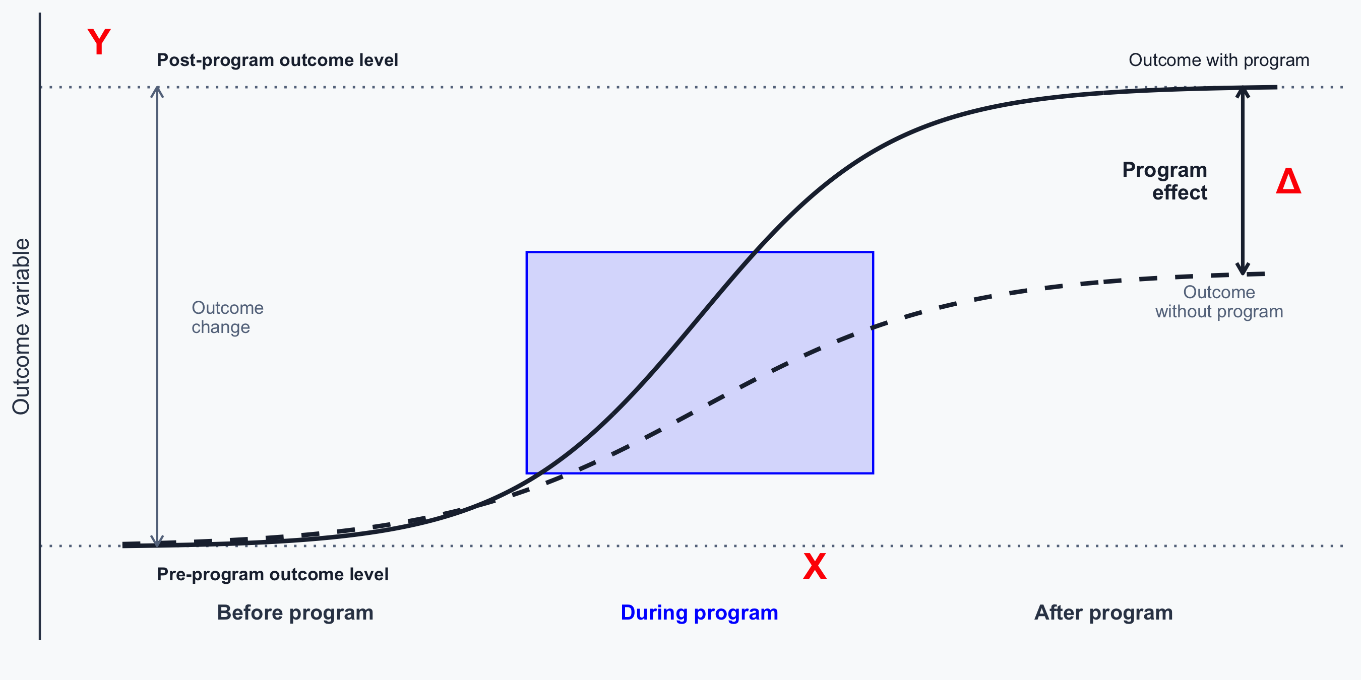
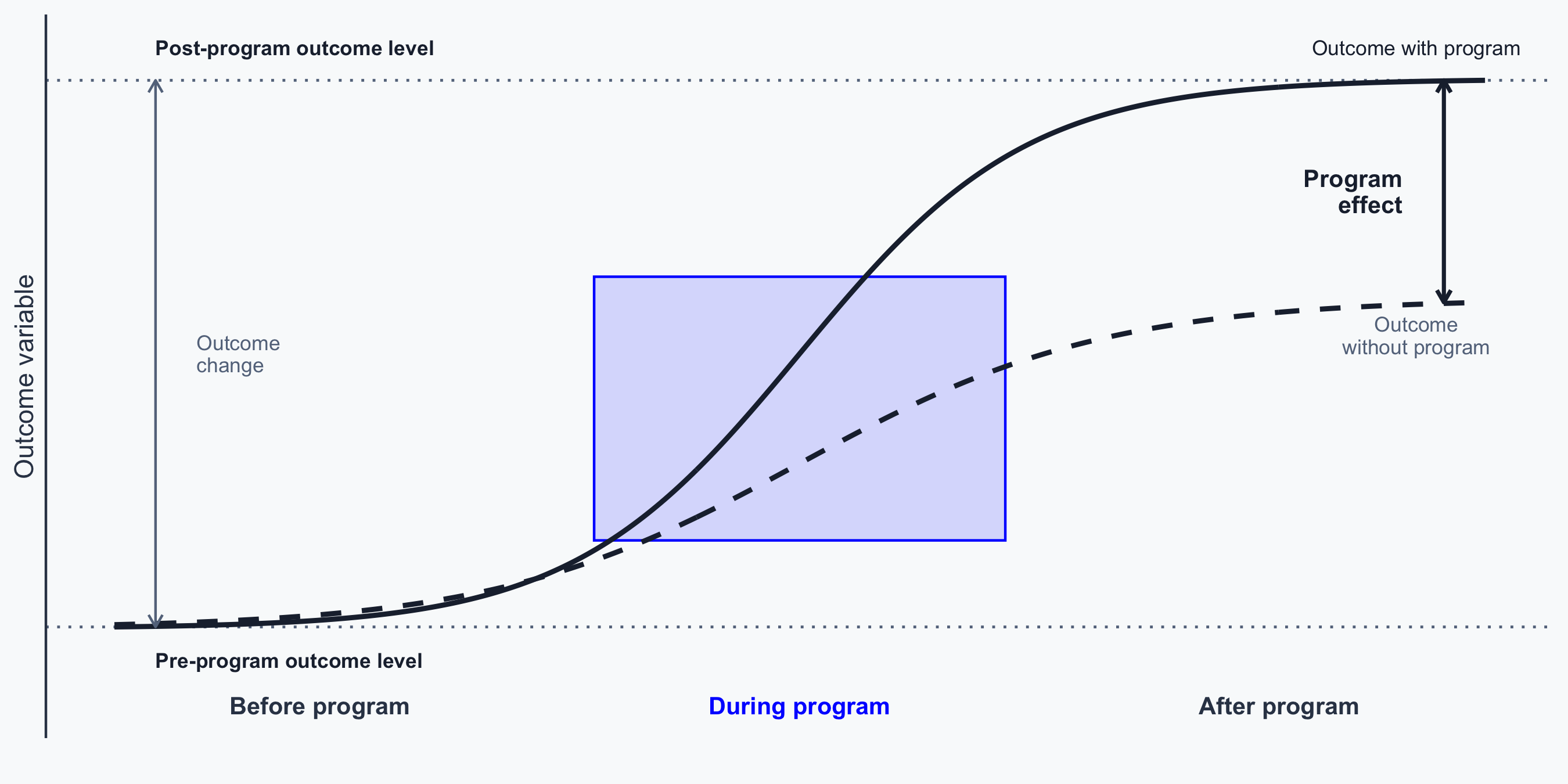
Outcomes and Programs

Types of Data

Experimental Data

Researcher controls which units get treated
Proving causation is easier

Observational Data

No control over which units get treated
Proving causation is harder

Causal Diagrams

What Is a DAG?

Directed Acyclic Graphs (DAGs):

Directed: arrows point from cause to effect
Acyclic: no cycles; arrows go one direction only
Graph: a visual representation of relationships

Why Use DAGs?

A DAG represents the theoretical model behind the data

Shows what to control for to identify causal effects

A causal effect is identified when confounders are removed

How to Draw a DAG

Four steps:

List all relevant variables
Simplify by grouping related variables
Connect with arrows using domain knowledge
Assess which paths need to be controlled

Step 1: List Variables

Example — factors affecting life expectancy:

GDP
Education
Public services
Health care
Urbanization
Conflict

Step 2: Simplify

Group related variables:

Health care \(\rightarrow\) subsumed under Public services
Crime rates \(\rightarrow\) subsumed under Conflict

Simplified: GDP, Education, Public services, Urbanization, Conflict

Steps 3–4: Connect Arrows

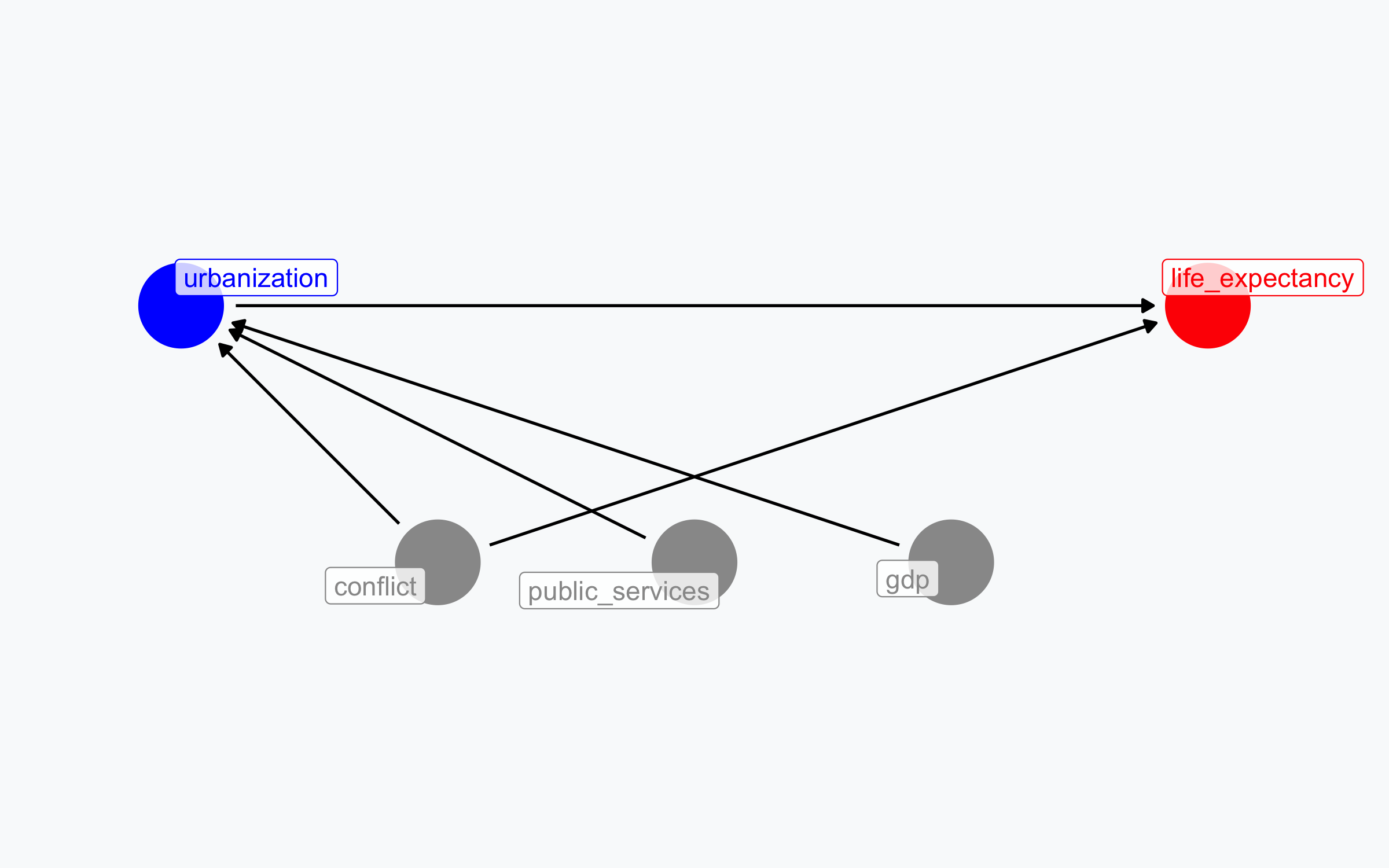
GDP, conflict, public services \(\rightarrow\) urbanization
Conflict also \(\rightarrow\) life expectancy directly

Causal Identification

Nodes connected by arrows are correlated
We care about the effect of urbanization on life expectancy

A causal effect is identified when the \(X \rightarrow Y\) link is isolated

DAG arrows help understand which paths to control

Types of Associations

Three Types of Associations

Type	Role of \(Z\)	Problem?
Confounding	\(Z\) causes both \(X\) and \(Y\)	Yes
Collision	\(X\) and \(Y\) both cause \(Z\)	Yes
Mediation	\(X \rightarrow Z \rightarrow Y\)	Helpful

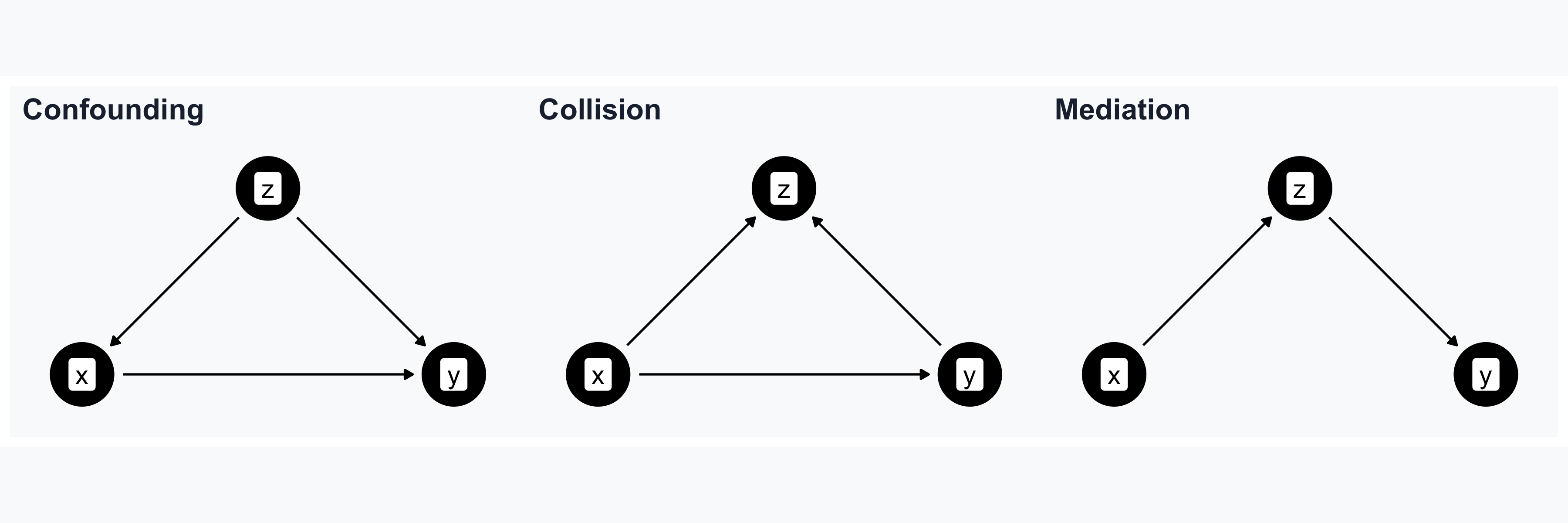
Confounding

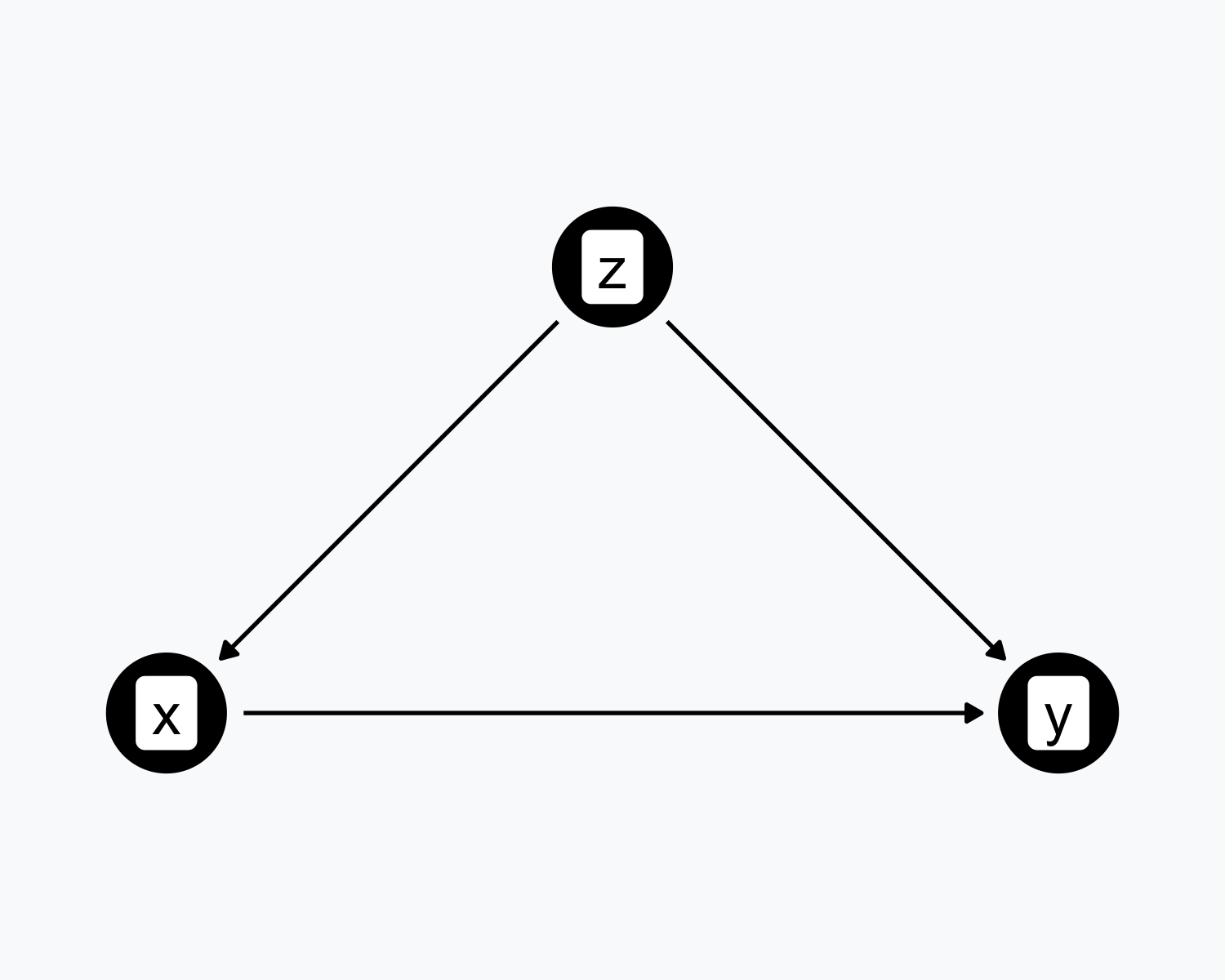
\(Z\) causes both \(X\) and \(Y\)
\(Z\) confounds the relationship between \(X\) and \(Y\)
The \(X \rightarrow Y\) relationship is not identified

Confounding Example

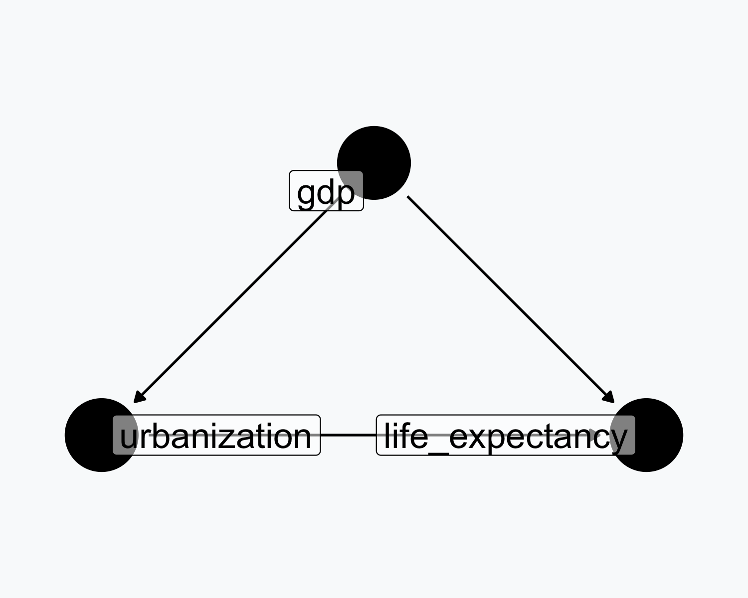
GDP causes both urbanization and life expectancy
GDP confounds the urbanization \(\rightarrow\) life expectancy link
Without controlling for GDP, the effect is biased

Confounding: Solutions

Include the confounder as a control in the regression
Matching: pair treated/untreated with similar \(Z\)
Stratifying: analyze within levels of \(Z\)

Most common approach: add \(Z\) to the regression

Confounding in Practice

# Bivariate: ignoring GDP (confounded)
mod_biv <- lm(life_expectancy ~ urbanization, data = final)
# Multivariate: controlling for GDP
mod_multi <- lm(life_expectancy ~ urbanization + log_gdp,
                data = final)

Confounding: The Coefficient Drops

Bivariate urbanization effect: 0.247
Multivariate urbanization effect: 0.055

The coefficient drops after controlling for GDP
GDP was inflating the apparent urbanization effect

This is what confounding looks like in practice

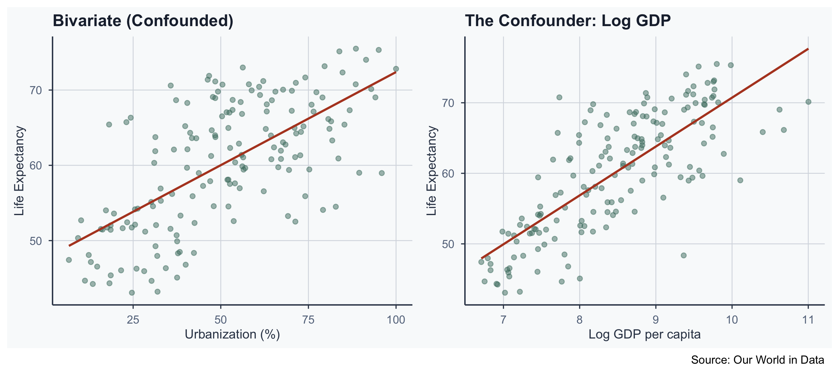
Confounding: Visualized

Collision

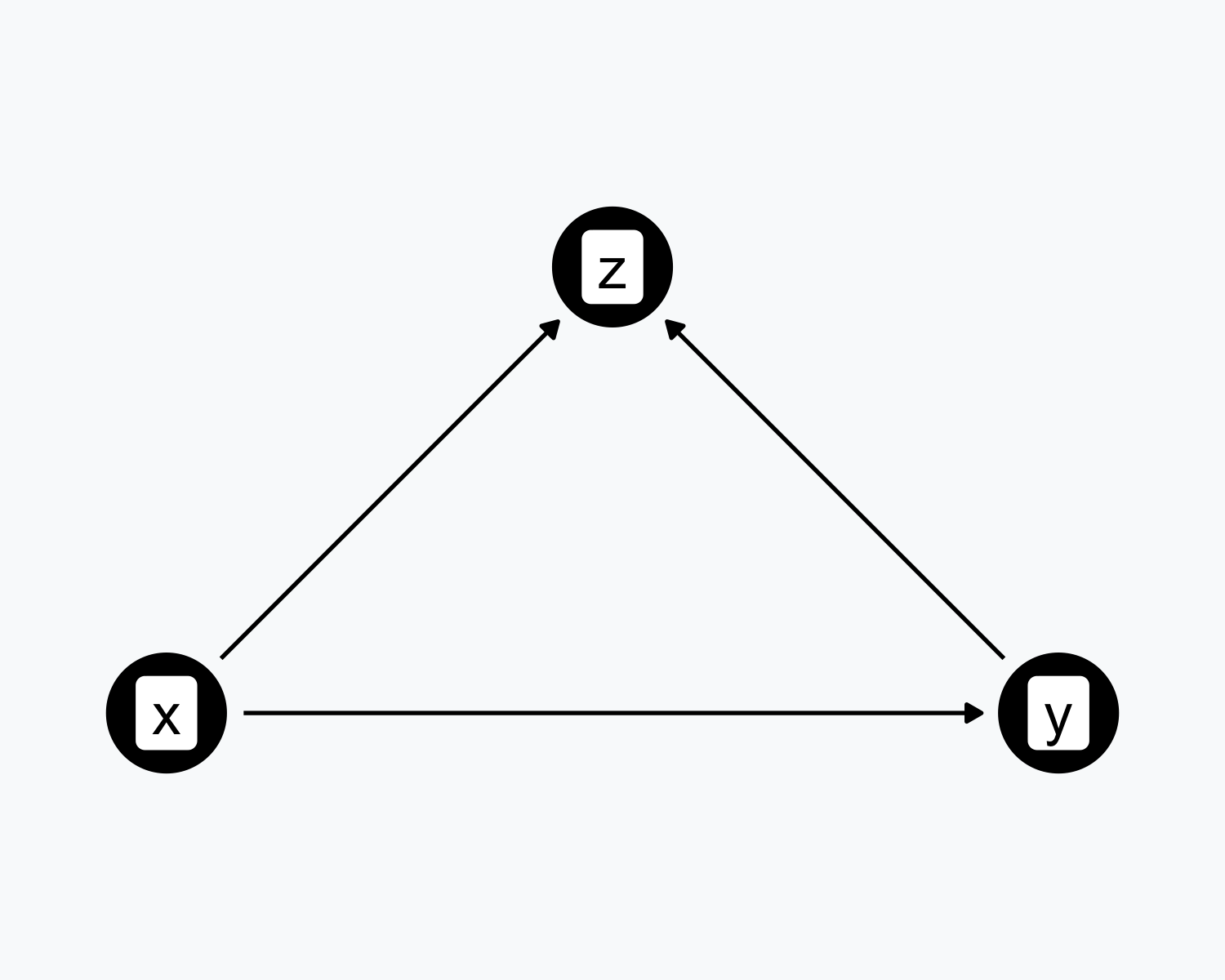
\(X\) and \(Y\) both cause \(Z\) (the collider)
Controlling for \(Z\) creates a spurious association

Collision Example

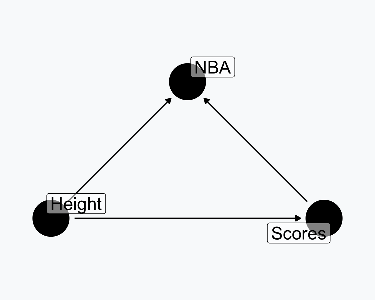
Height and scoring both cause NBA recruitment
Controlling for NBA status creates a false link

Collision: Solutions

Collect additional data beyond the collider group
- Include both NBA and non-NBA players

Restrict the sample to avoid conditioning on \(Z\)
- Analyze only non-NBA players

Key rule: do not control for colliders

Mediation

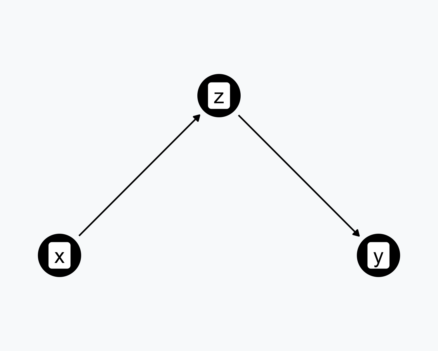
\(X\) causes \(Z\), and \(Z\) causes \(Y\)
\(Z\) is a mediator on the causal path

Mediation Example

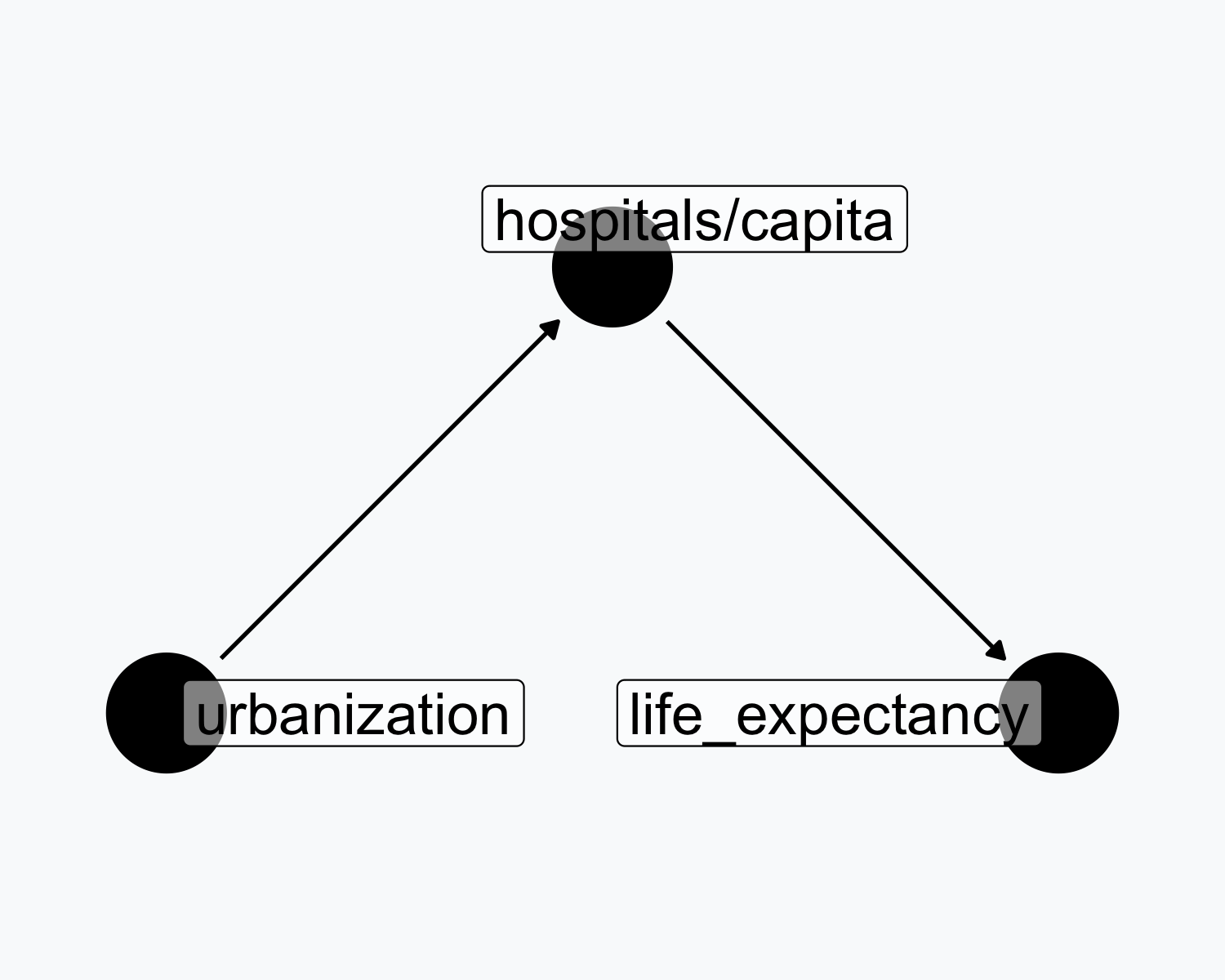
Urbanization \(\rightarrow\) hospitals/capita \(\rightarrow\) life expectancy
Hospitals mediate the urbanization effect

Testing for Mediation

Run four regressions:

\(Y = \beta_0 + \beta_1 X + \epsilon\)
\(M = \beta_0 + \beta_1 X + \epsilon\)
\(Y = \beta_0 + \beta_1 M + \epsilon\)
\(Y = \beta_0 + \beta_1 X + \beta_2 M + \epsilon\)

If \(X\) becomes insignificant in (4): full mediation
If \(X\) is reduced but significant: partial mediation

Full vs. Partial Mediation

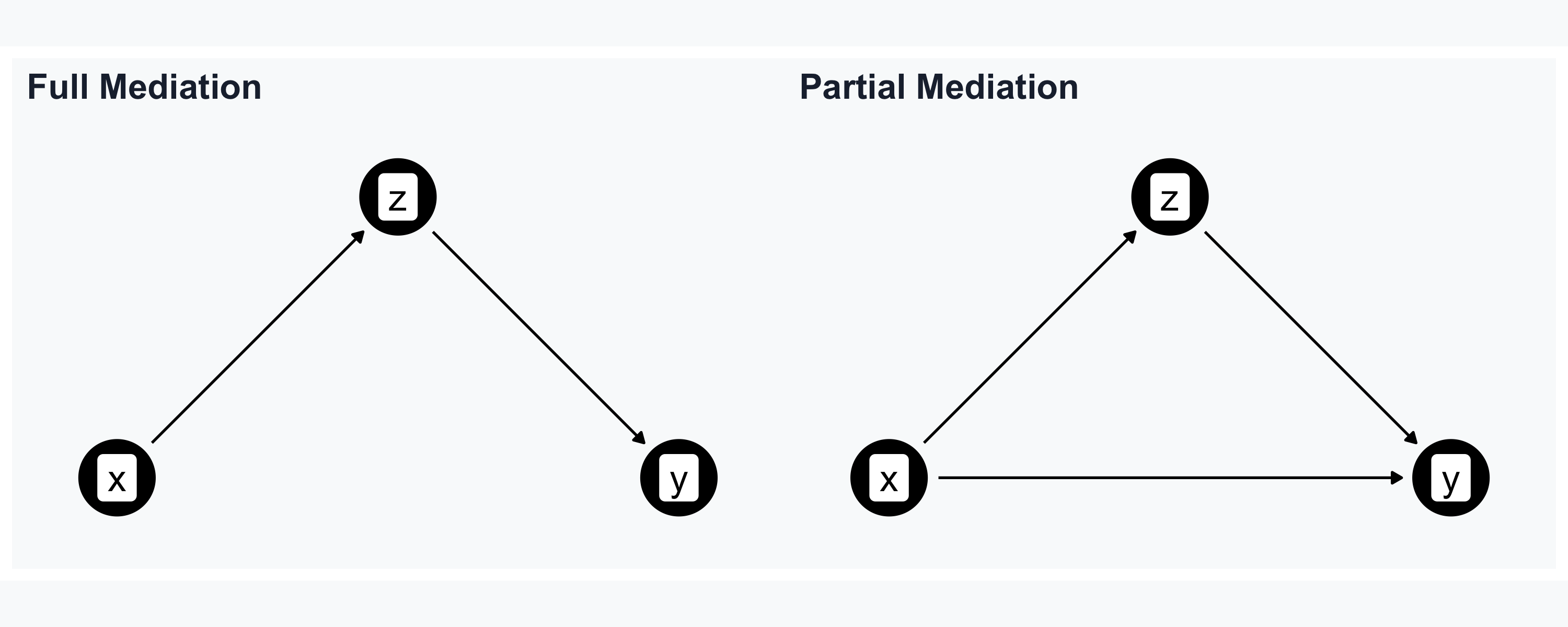
Full: all of \(X\)’s effect passes through \(Z\)
Partial: \(X\) affects \(Y\) directly and through \(Z\)

Summary of Variable Relationships

Causality

Causality Notation

We write the causal effect as:

\[E(Y \mid X = x)\]

“Expected value of \(Y\), given that \(X\) takes value \(x\)”

Examples:

\(E(\text{life expectancy} \mid \text{+1 pct. pt. urbanization})\)
\(E(\text{income} \mid \text{+1 year of education})\)
\(E(\text{malaria risk} \mid \text{insecticide-treated net})\)

Causality in RCTs

In RCTs, we control who gets treated — confounders vanish

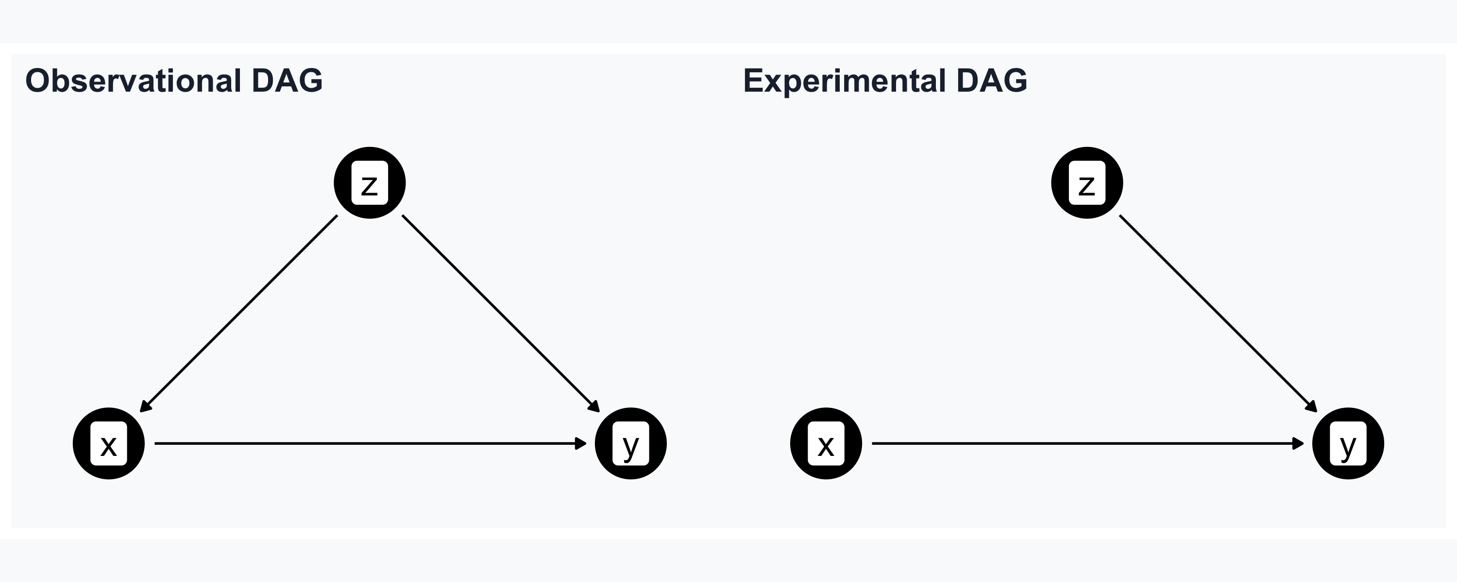
Randomization breaks the arrow from \(Z\) to \(X\)

Correlation \(\neq\) Causation

\[P(Y \mid X = x) \neq P(Y \mid X)\]

\(P(Y \mid X)\) gives a correlation, not a causal effect
A simple regression captures association, not causation

Causal identification requires controlling confounders or randomization

Potential Outcomes Framework

The Counterfactual Problem

Potential Outcomes Notation

In a treatment vs. control setting:

\[\Delta = E(Y \mid X = 1) - E(Y \mid X = 0)\]

\(Y^1_i\): outcome for individual \(i\) if treated
\(Y^0_i\): outcome for individual \(i\) if untreated
\(\Delta_i = Y^1_i - Y^0_i\): individual treatment effect

The Fundamental Problem

We can never observe both potential outcomes for one person:

\[\Delta_i = Y^1_i - \text{ ?}\]

A patient either takes the pill or does not
We cannot observe the counterfactual
This is the fundamental problem of causal inference

What We Would Like

Patient	Treatment	Outcome 1	Outcome 2
1	1	\(Y_1\) (Treated)	\(Y_1\) (Untreated)
2	0	\(Y_2\) (Treated)	\(Y_2\) (Untreated)
3	1	\(Y_3\) (Treated)	\(Y_3\) (Untreated)
4	1	\(Y_4\) (Treated)	\(Y_4\) (Untreated)
5	0	\(Y_5\) (Treated)	\(Y_5\) (Untreated)

What We Actually Observe

Patient	Treatment	Outcome 1	Outcome 2
1	1	\(Y_1\) (Treated)	???
2	0	???	\(Y_2\) (Untreated)
3	1	\(Y_3\) (Treated)	???
4	1	\(Y_4\) (Treated)	???
5	0	???	\(Y_5\) (Untreated)

We only see one potential outcome per person
The other is the missing counterfactual

Average Treatment Effects

ATT and ATU

We compute group averages from what we observe:

Average Treatment on the Treated (ATT):

\[ATT = \bar{Y}_T \mid X = 1\]

Average Treatment on the Untreated (ATU):

\[ATU = \bar{Y}_U \mid X = 0\]

Average Treatment Effect (ATE)

Combine ATT and ATU:

\[ATE = ATT - ATU\]

ATE estimates the average causal effect of treatment
But it may contain selection bias

Selection Bias

\[ATE = (ATT - ATU) + \text{Selection Bias}\]

Confounders and colliders cause selection bias
In an RCT, selection bias \(= 0\) due to randomization

Without randomization, ATE \(\neq\) true causal effect

Example: Bocconi vs. JCU

Effect of graduating from Bocconi on monthly income?

Student	Bocconi	Income
1	1	2,400
2	0	2,000
3	1	2,500
4	1	2,800
5	0	2,100
6	0	2,000
7	0	2,200

Computing the ATE

\[ATT = \frac{2400 + 2500 + 2800}{3} \approx 2567\]

\[ATU = \frac{2000 + 2100 + 2000 + 2200}{4} = 2075\]

\[ATE \approx 2567 - 2075 = 492\]

But this is an observational study
\(492 = (ATT - ATU) + \text{Selection Bias}\)

Selection Bias in the Example

Why might there be selection bias?

Students choosing Bocconi may prefer finance/economics
These fields tend to have higher incomes

The “Bocconi effect” is confounded by career preferences
We cannot isolate the true university effect

Randomization

Why Randomize?

Randomization makes treatment independent of potential outcomes:

\[X \perp\!\!\!\perp Y^1, Y^0\]

Mean potential outcomes are identical across groups
Selection bias \(= 0\)

ATE equals the observed difference in group means

What Randomization Ensures

Treated and untreated groups are comparable
- Same average height, income, education, etc.

Differences in outcomes are caused by treatment
Not by pre-existing differences between groups

Internal & External Validity

Internal validity: findings are reliable for the sample

External validity: findings generalize to the population

RCTs have strong internal validity
External validity depends on sample representativeness

Conclusion

Summary

Programs: inputs \(\rightarrow\) activities \(\rightarrow\) outputs \(\rightarrow\) outcomes
DAGs: directed acyclic graphs map causal structure
Confounding: \(Z\) causes both \(X\) and \(Y\); control for \(Z\)
Potential outcomes: the counterfactual we cannot observe
ATE \(=\) ATT \(-\) ATU; may include selection bias
Randomization: eliminates selection bias in RCTs