Working with Data in R
Dataframes, Lists, External Files, Paths
What You’ll Learn Today
- Creating and Subsetting Dataframe
- Loading External files:
.csvand.xlsx - Relative vs. Absolute Paths
- Handling file or directory errors
- Examining entries in a dataframe
Using R
Using R
Using R
Using R
Using R
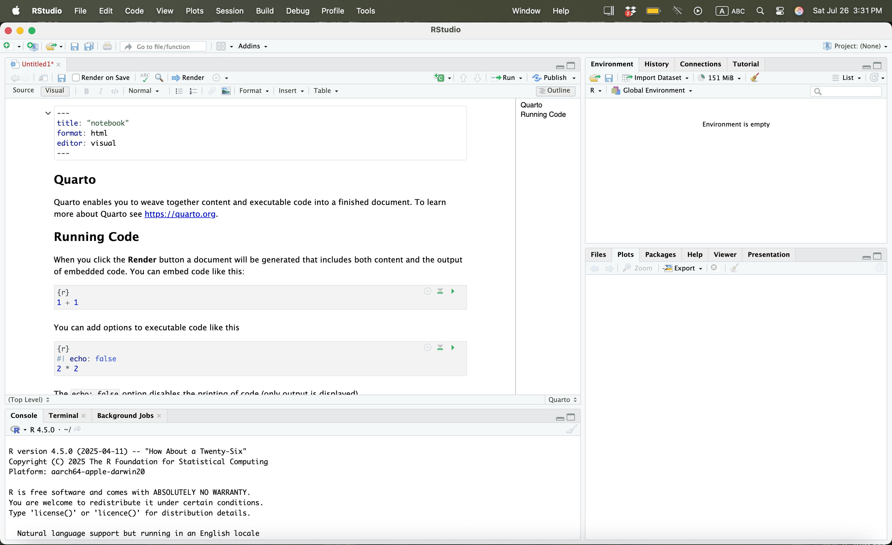
Using R
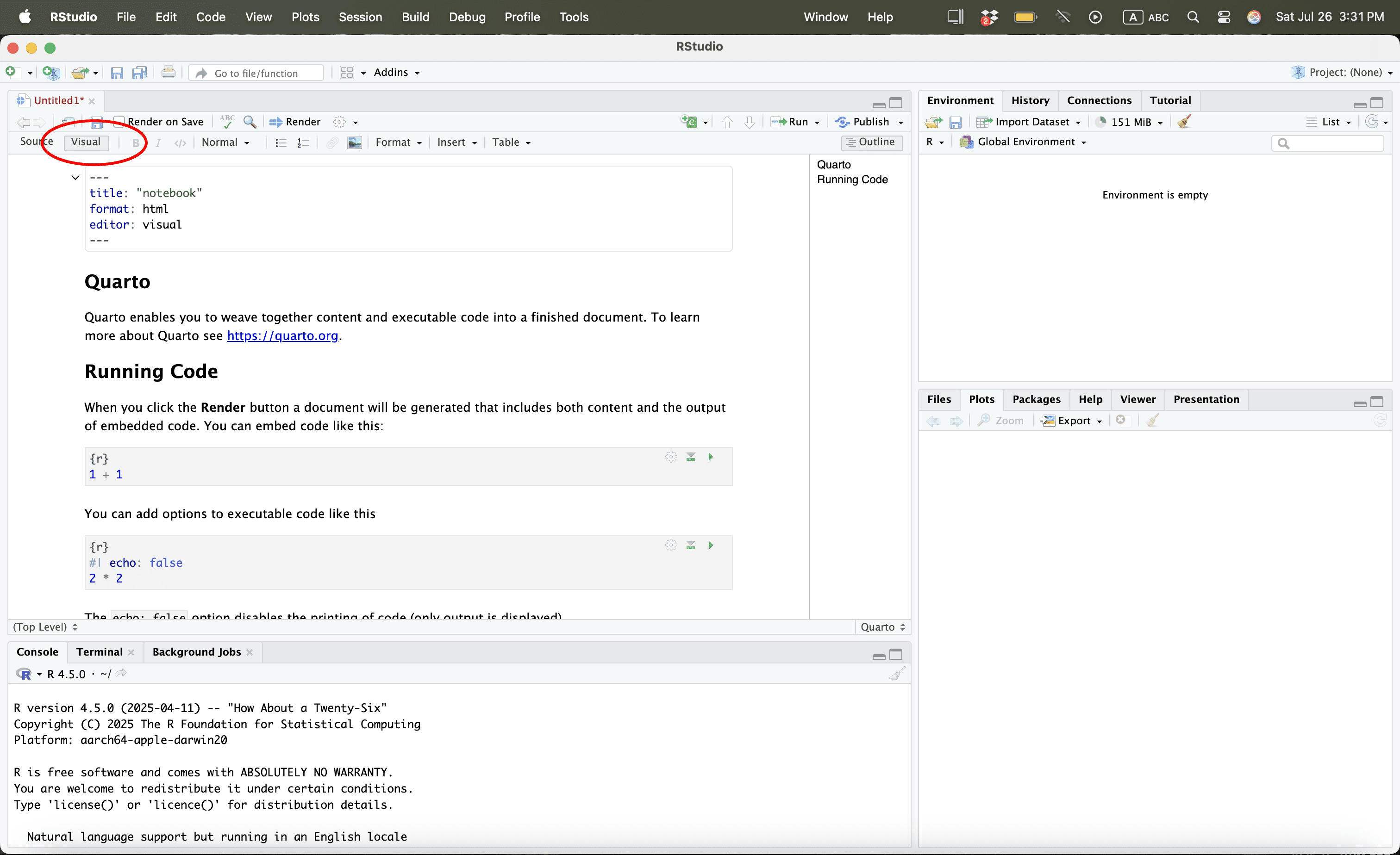
Using R
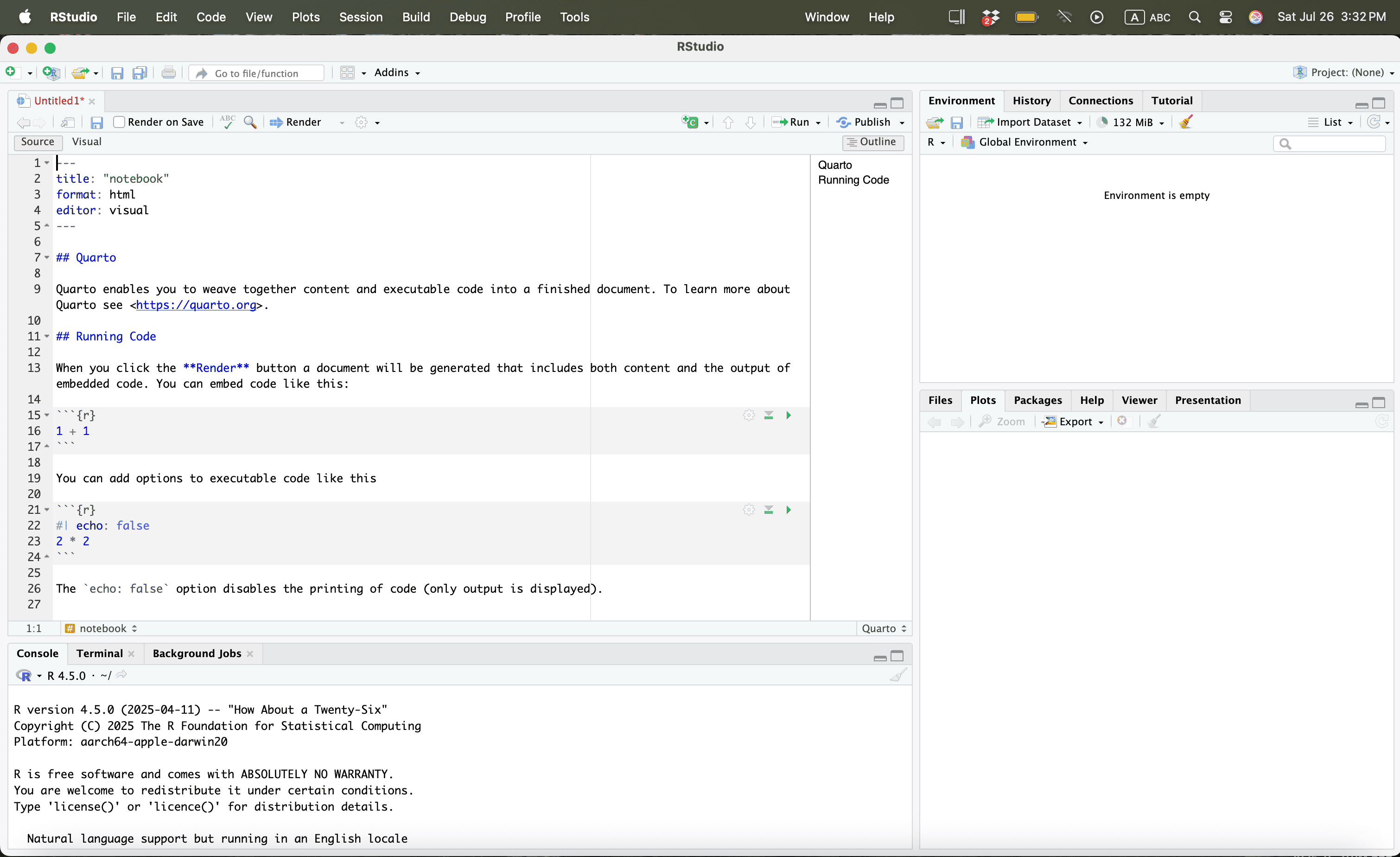
Using R
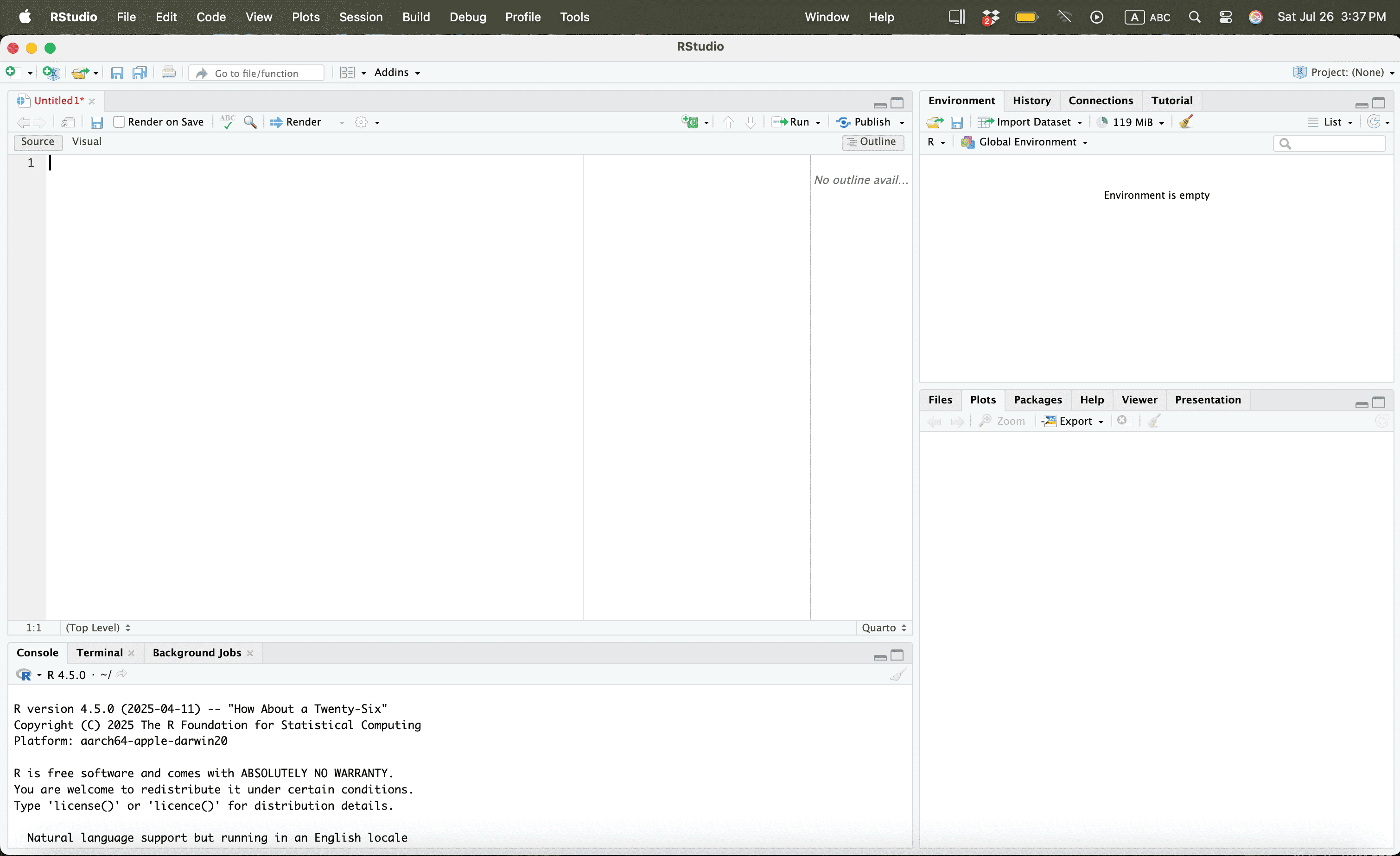
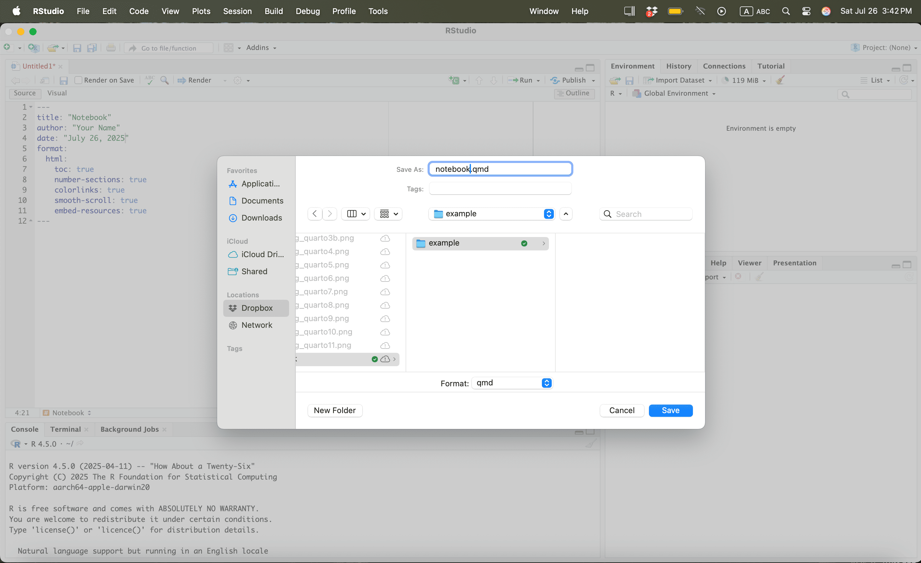
Press CMD + A or Ctrl + A and then Press Delete
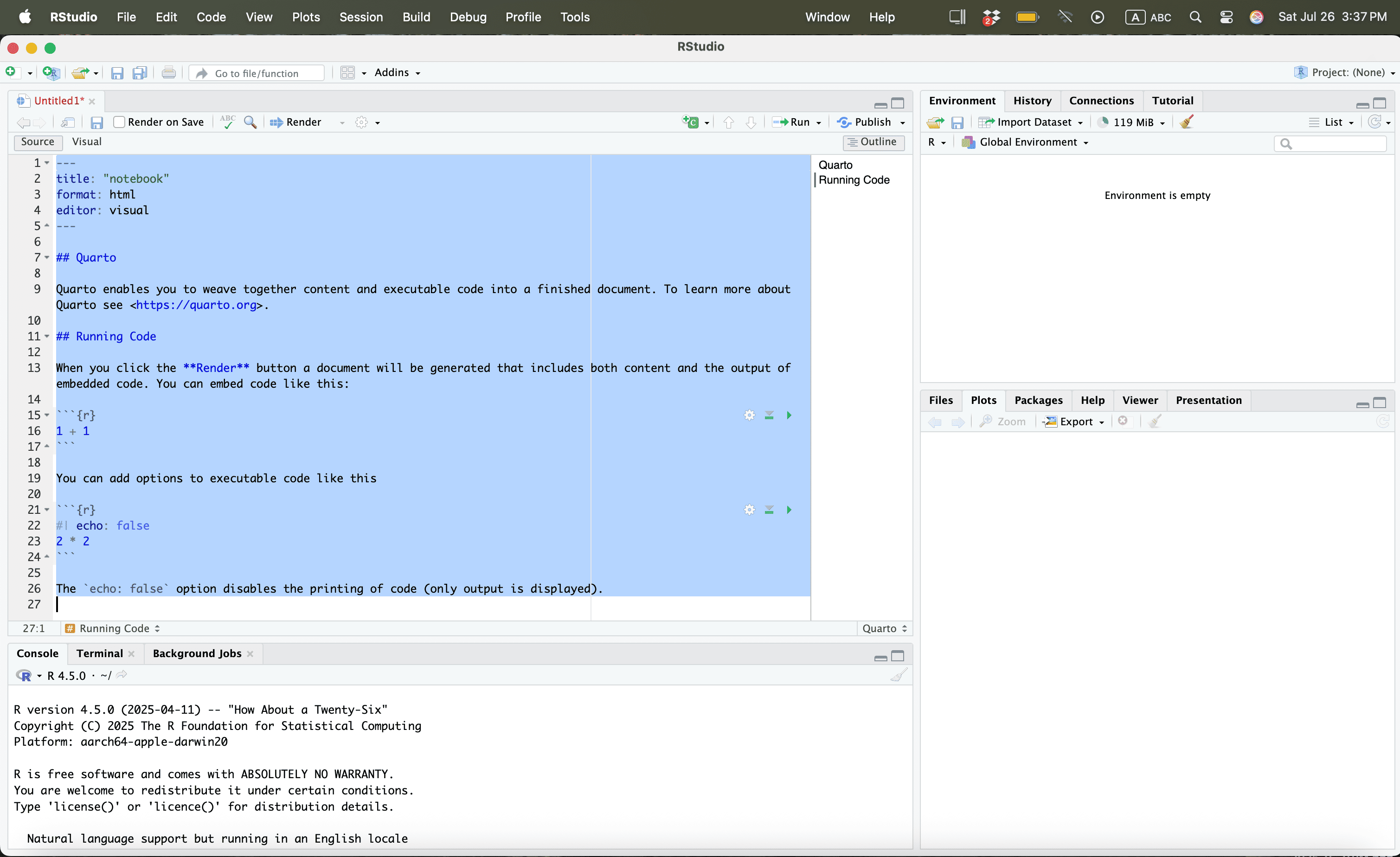
Using R
Using R
Then type:
Using R

Using R
Using R
Using R
Using R
Using R
Using R
Using R

Using R

Using R
Using R
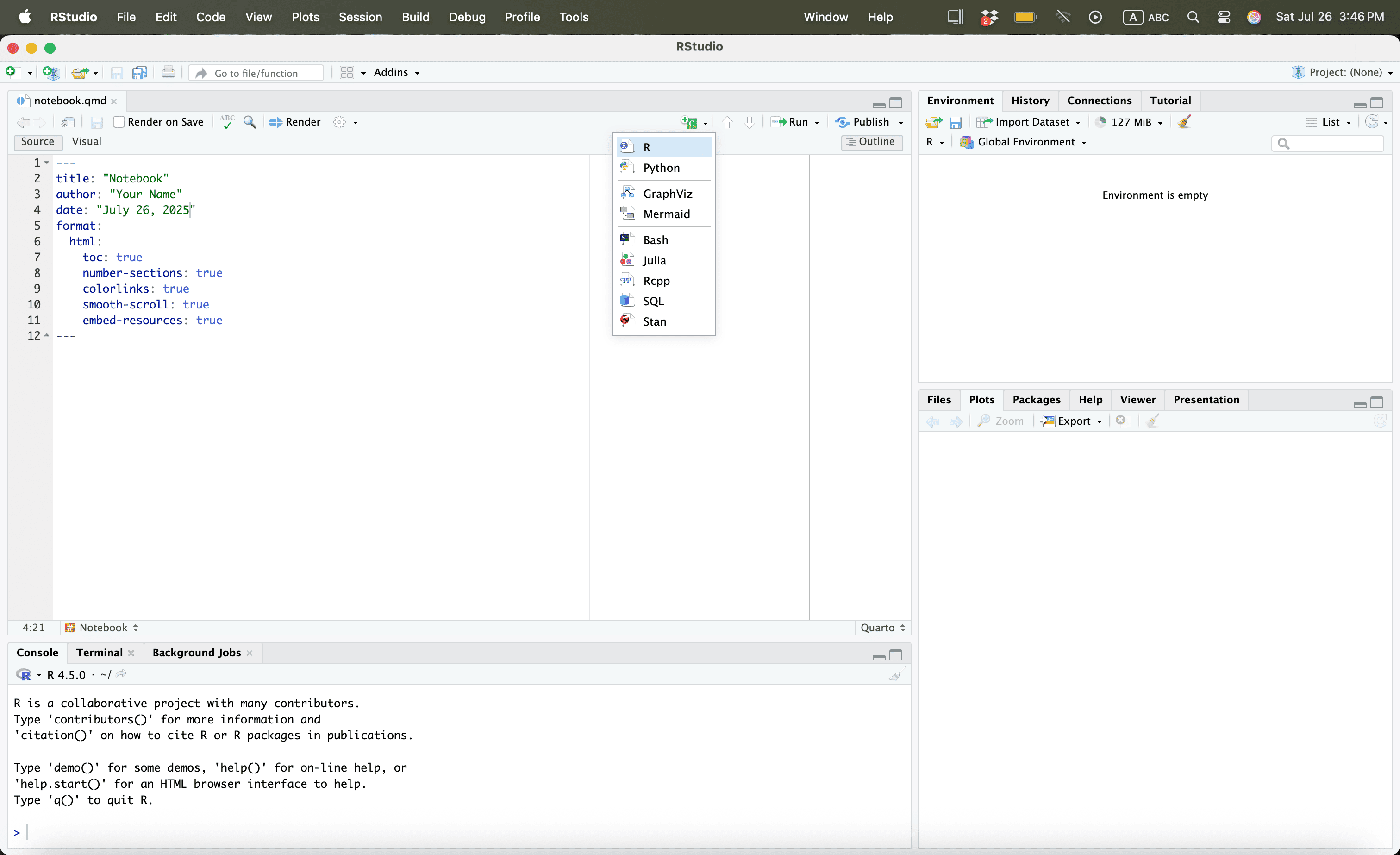
Using R
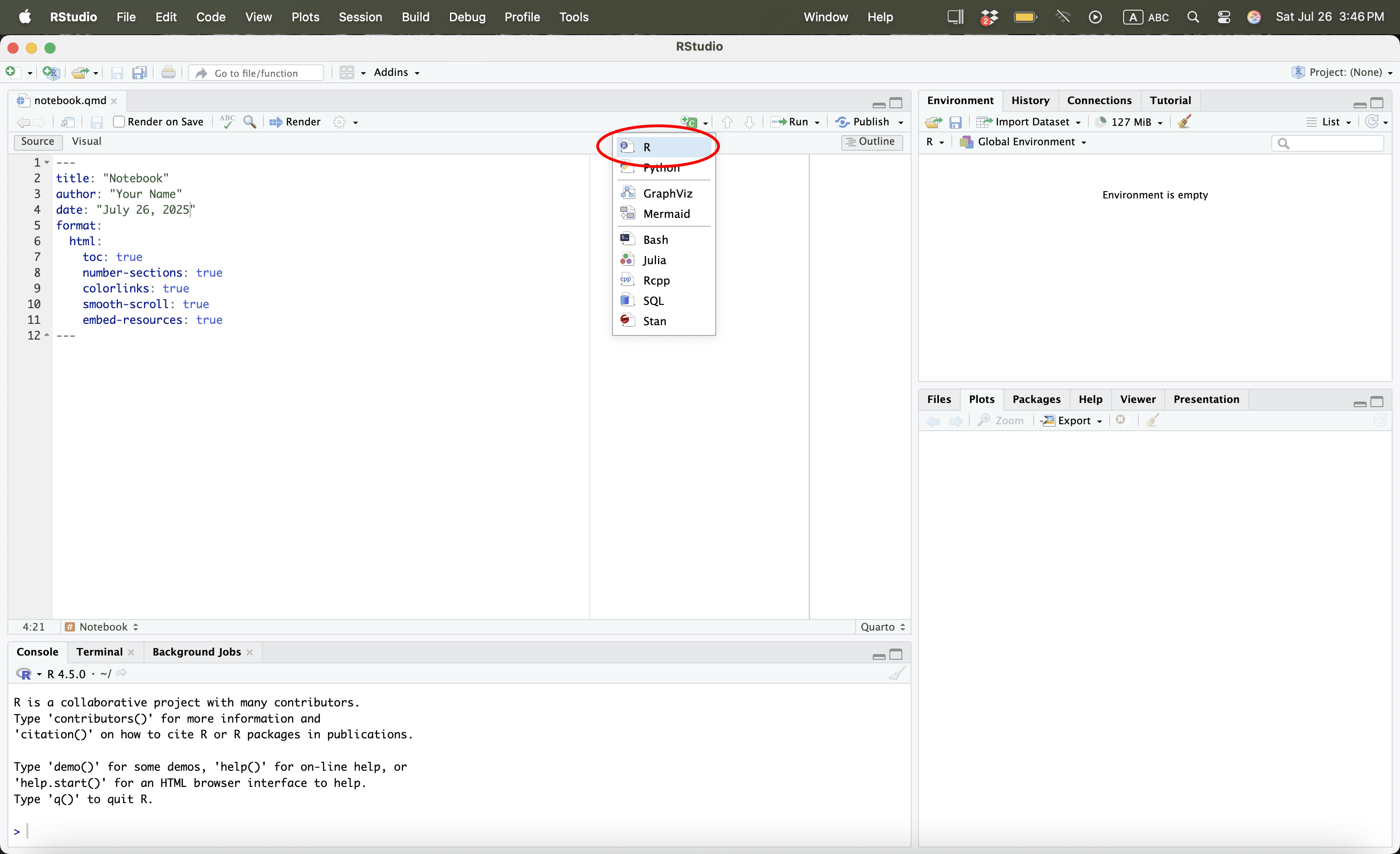
Using R
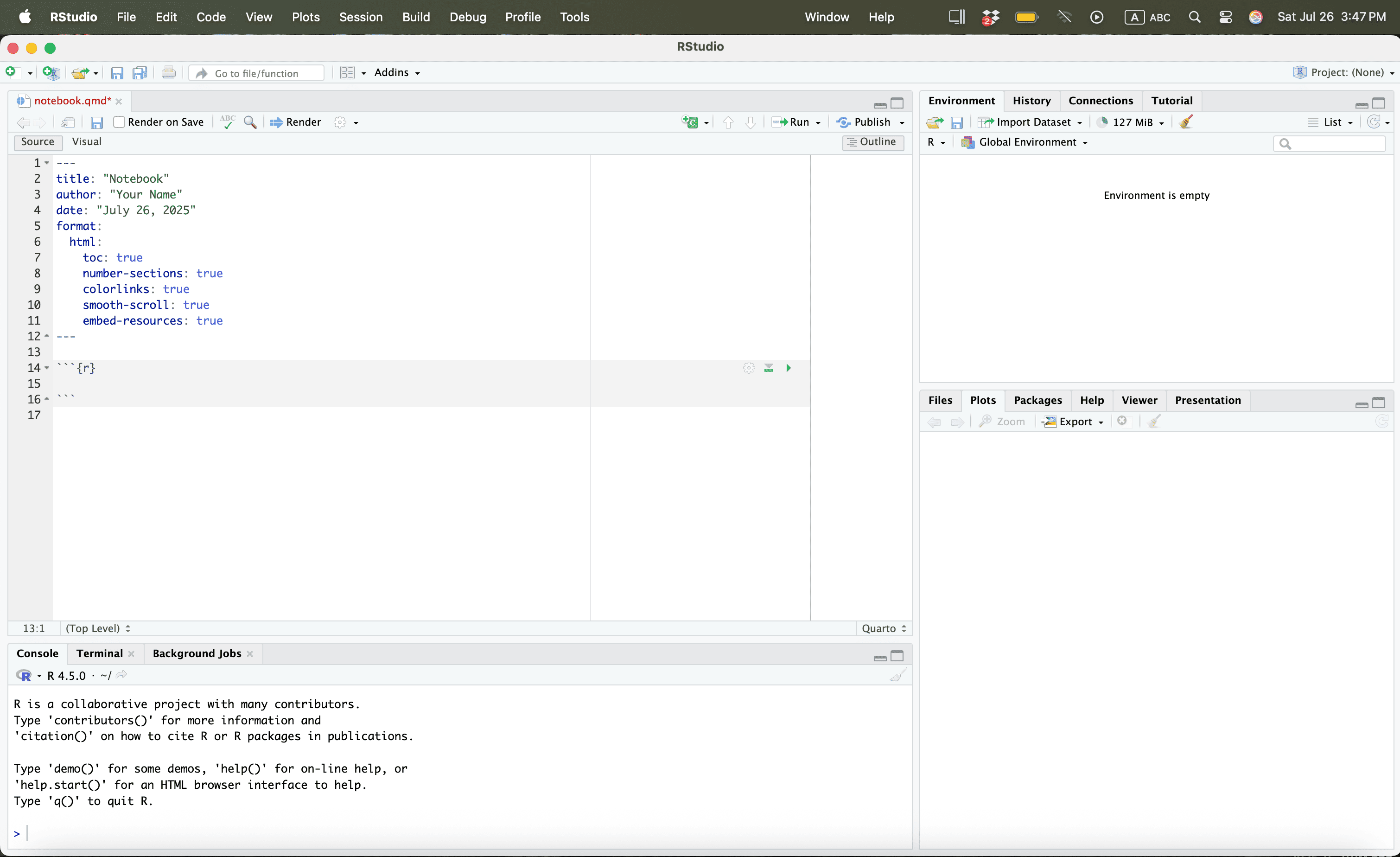
Using R
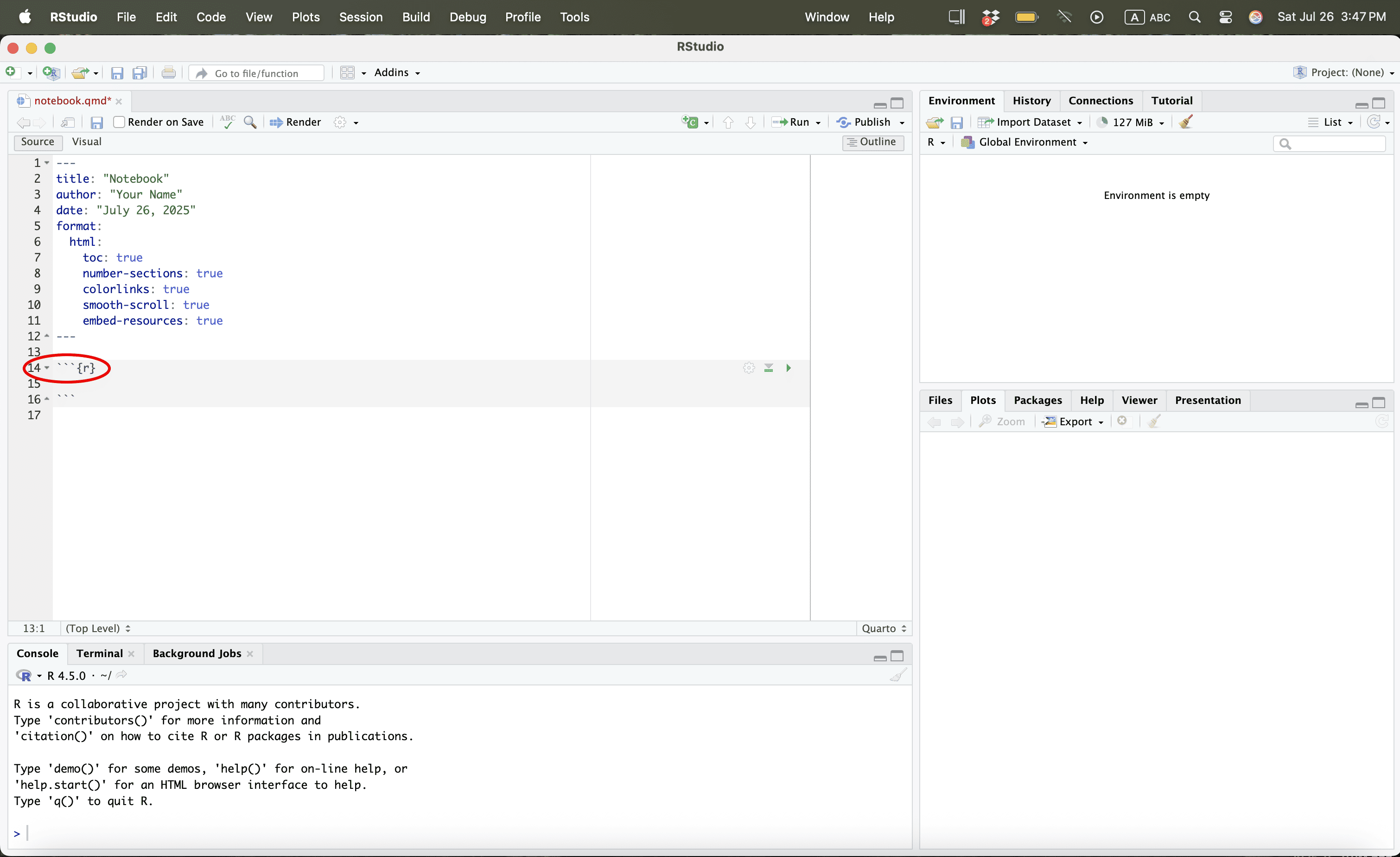
Using R
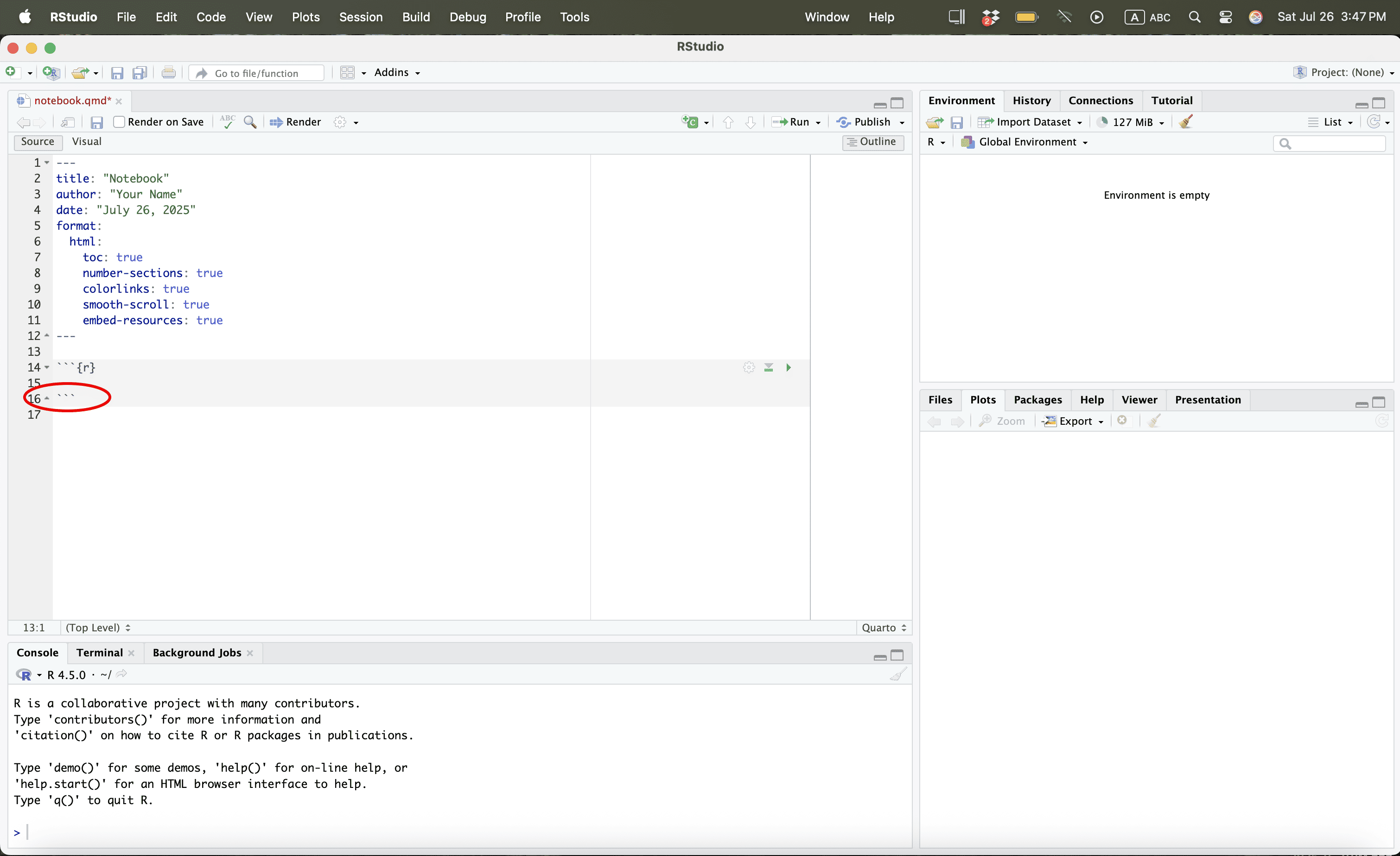
Using R
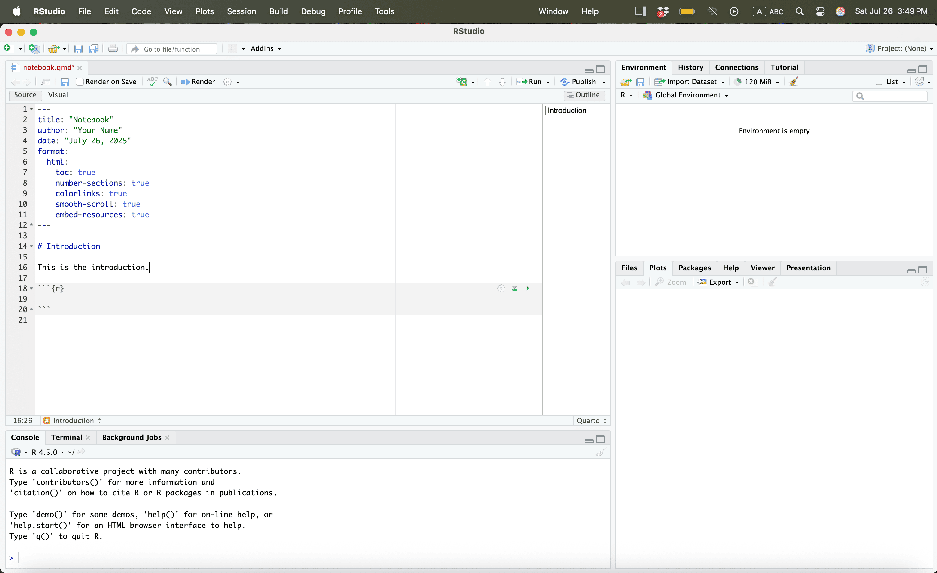
Using R
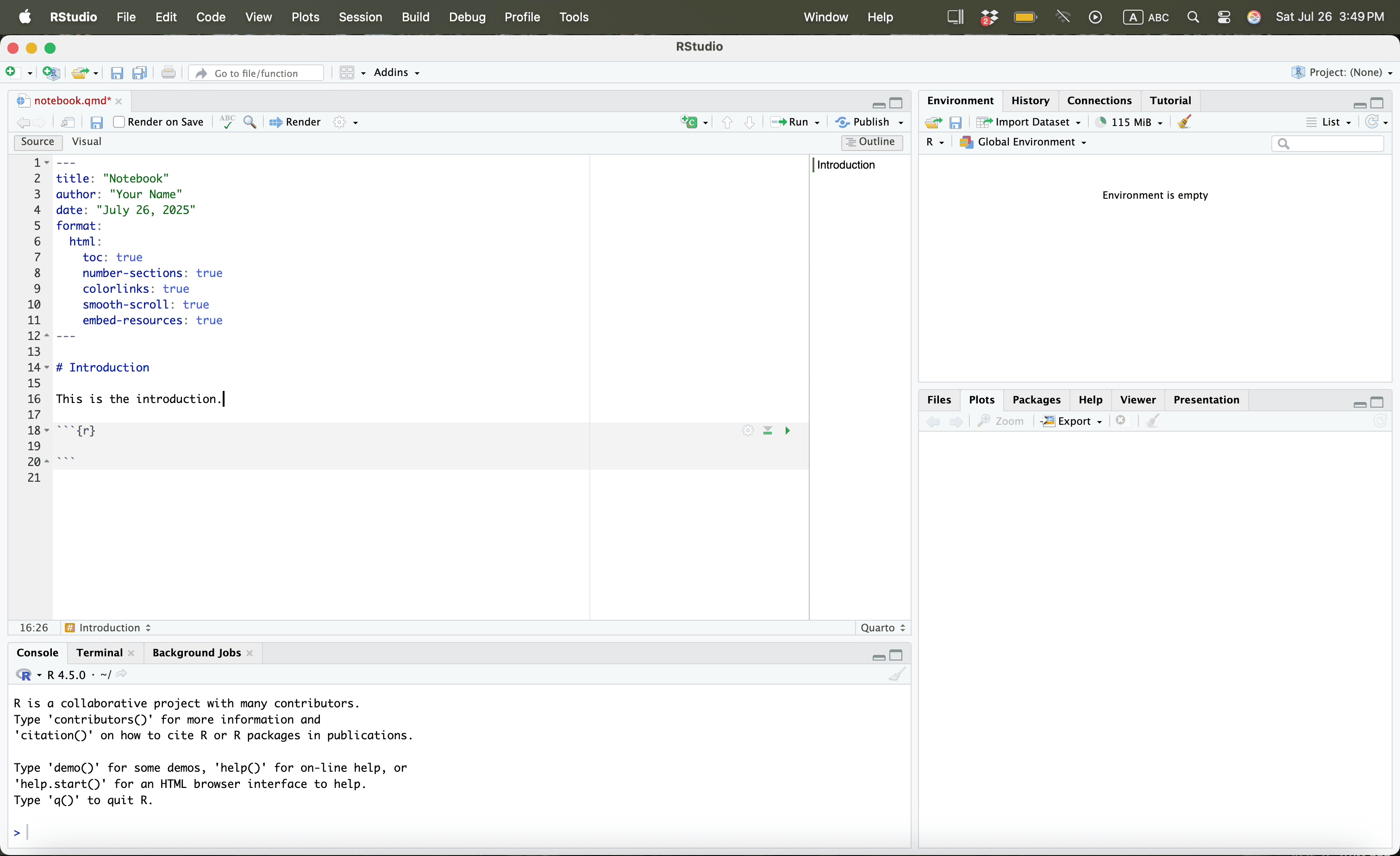
Using R
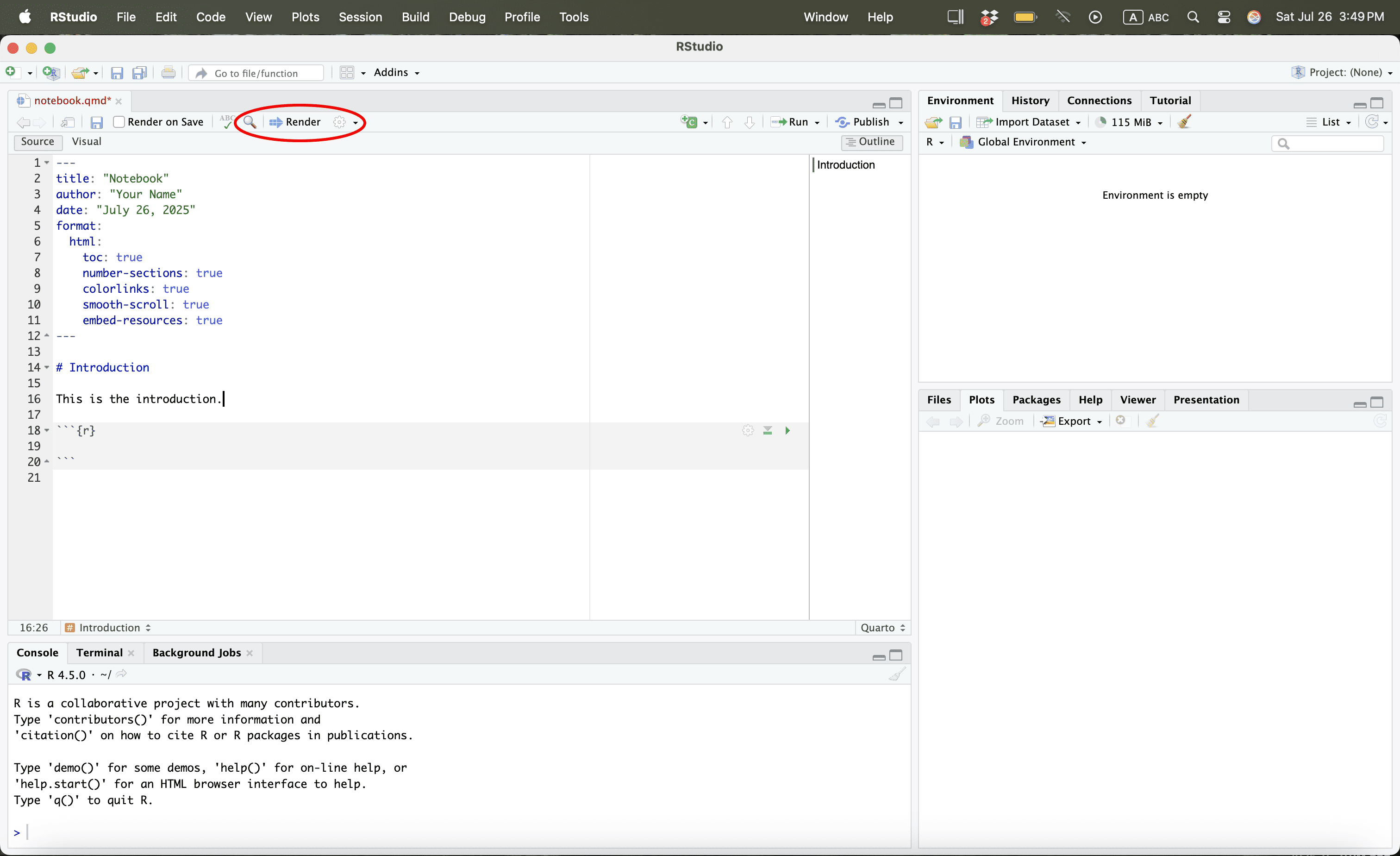
Using R
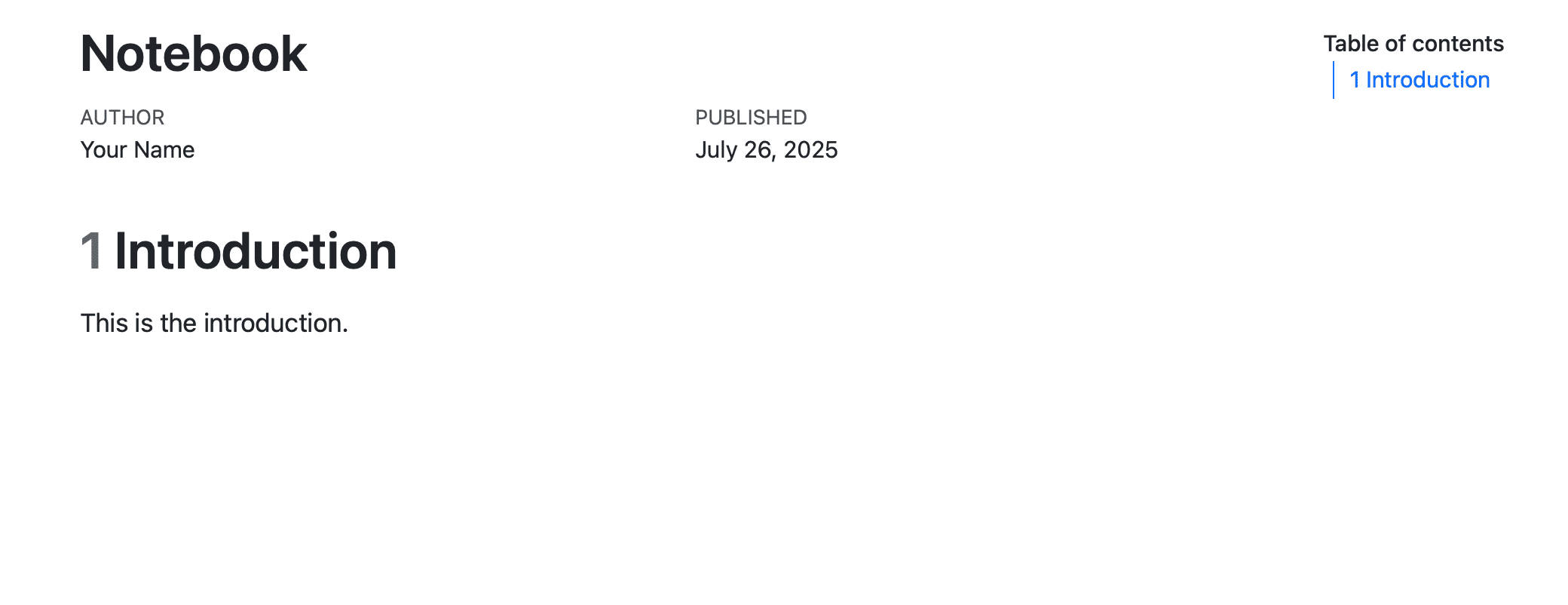
Using R
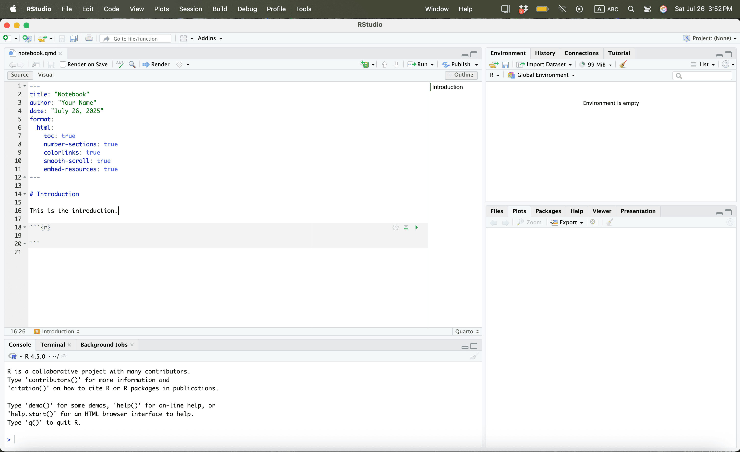
Using R
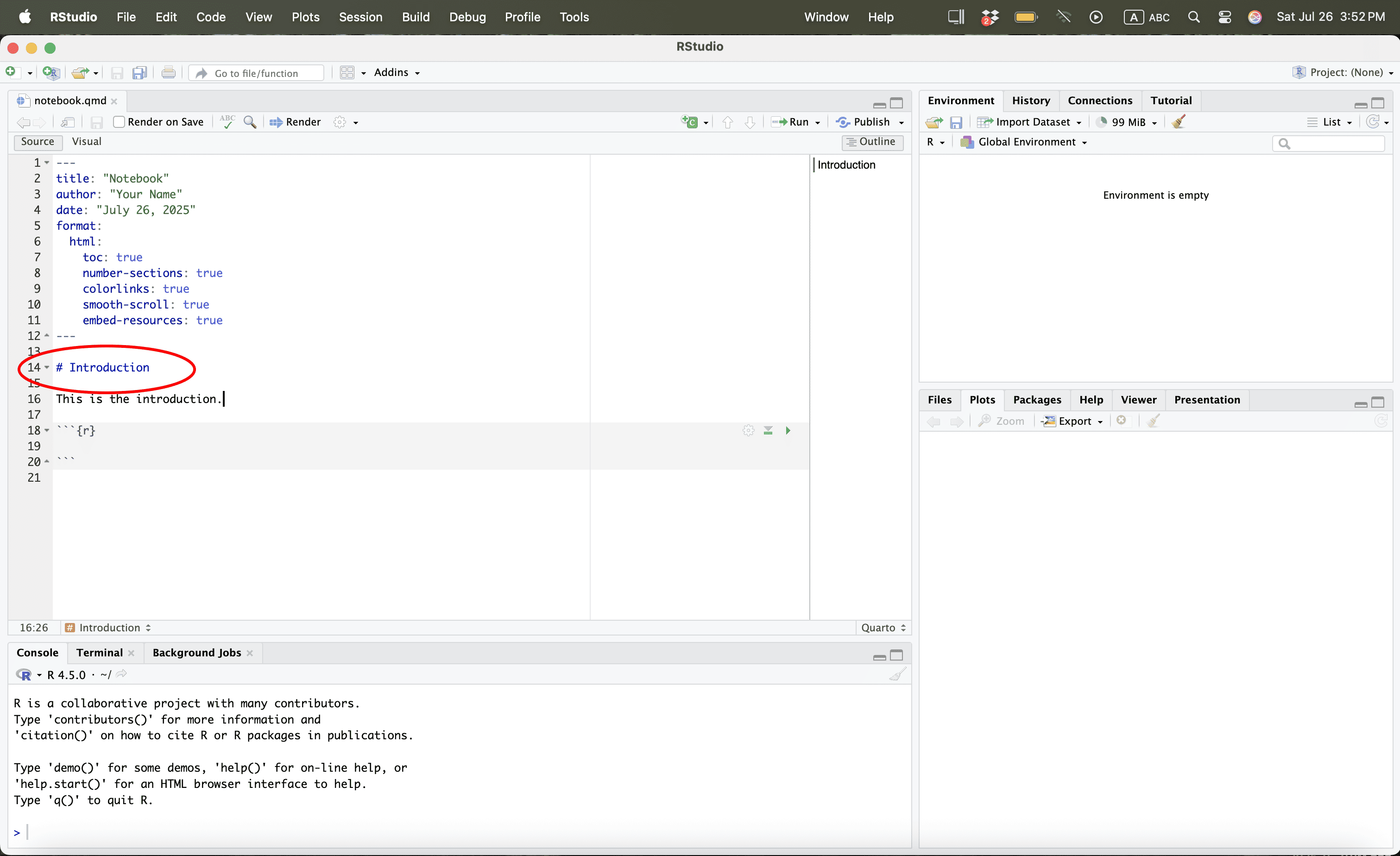
Using R
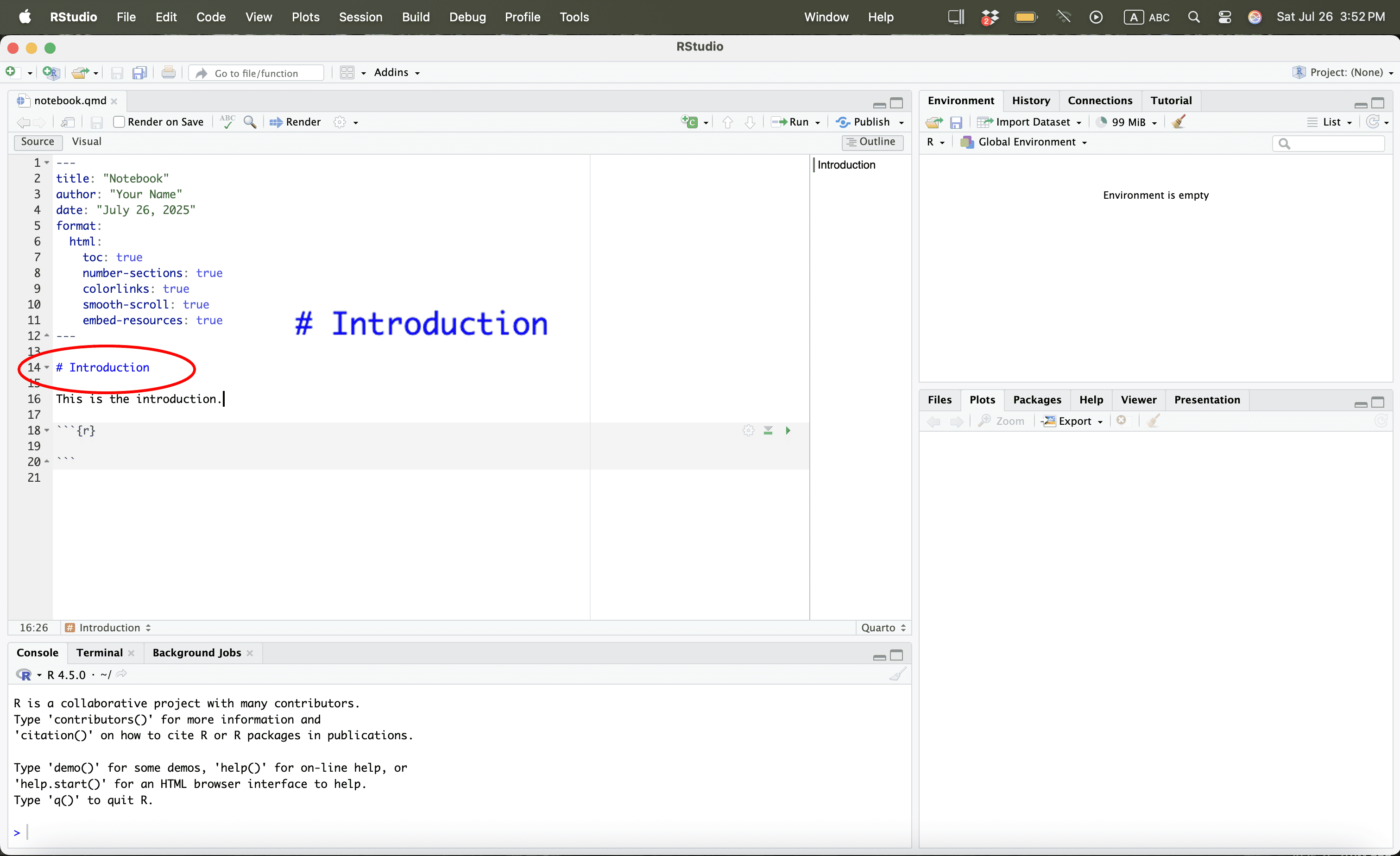
Using R
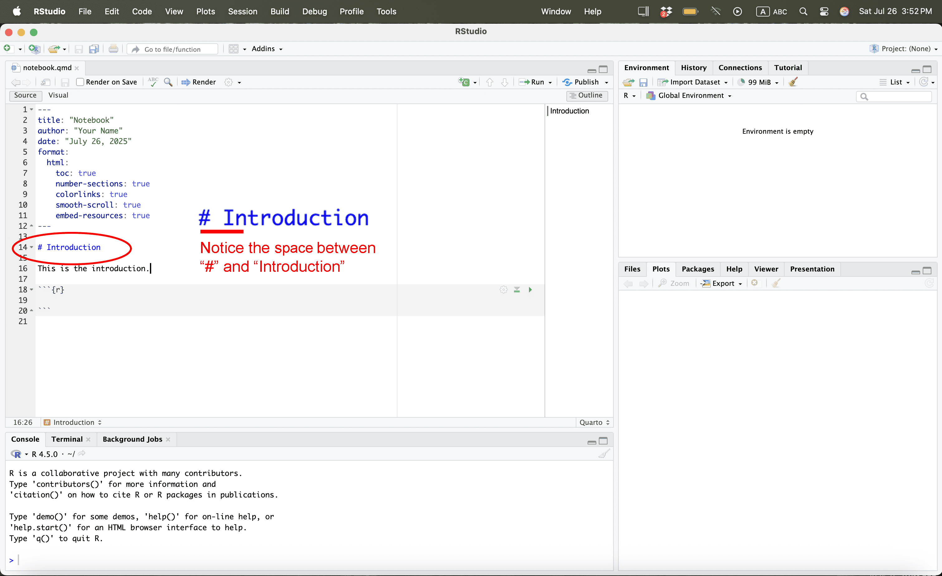
Creating a Dataframe
Creating a Dataframe
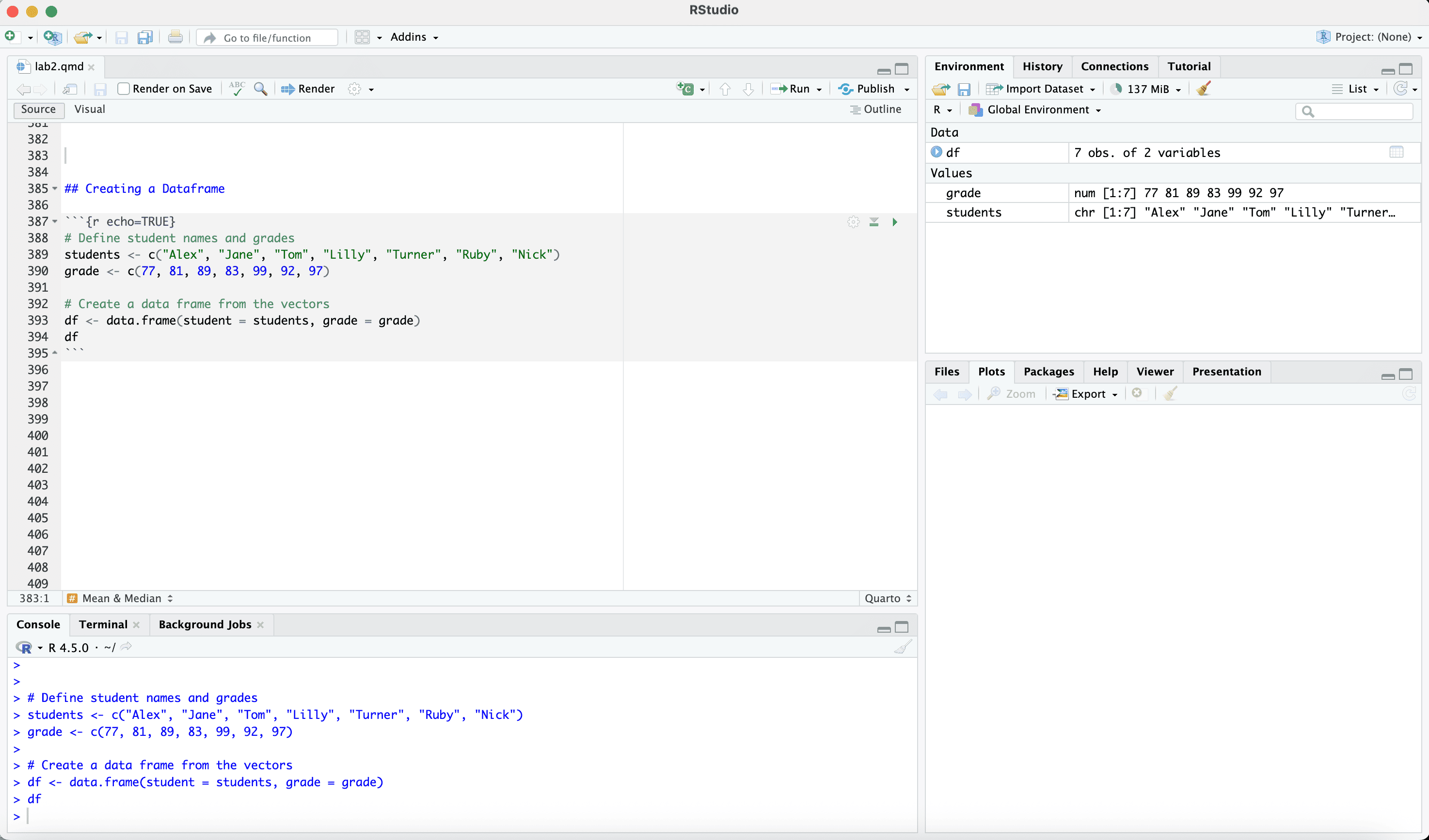
Creating a Dataframe
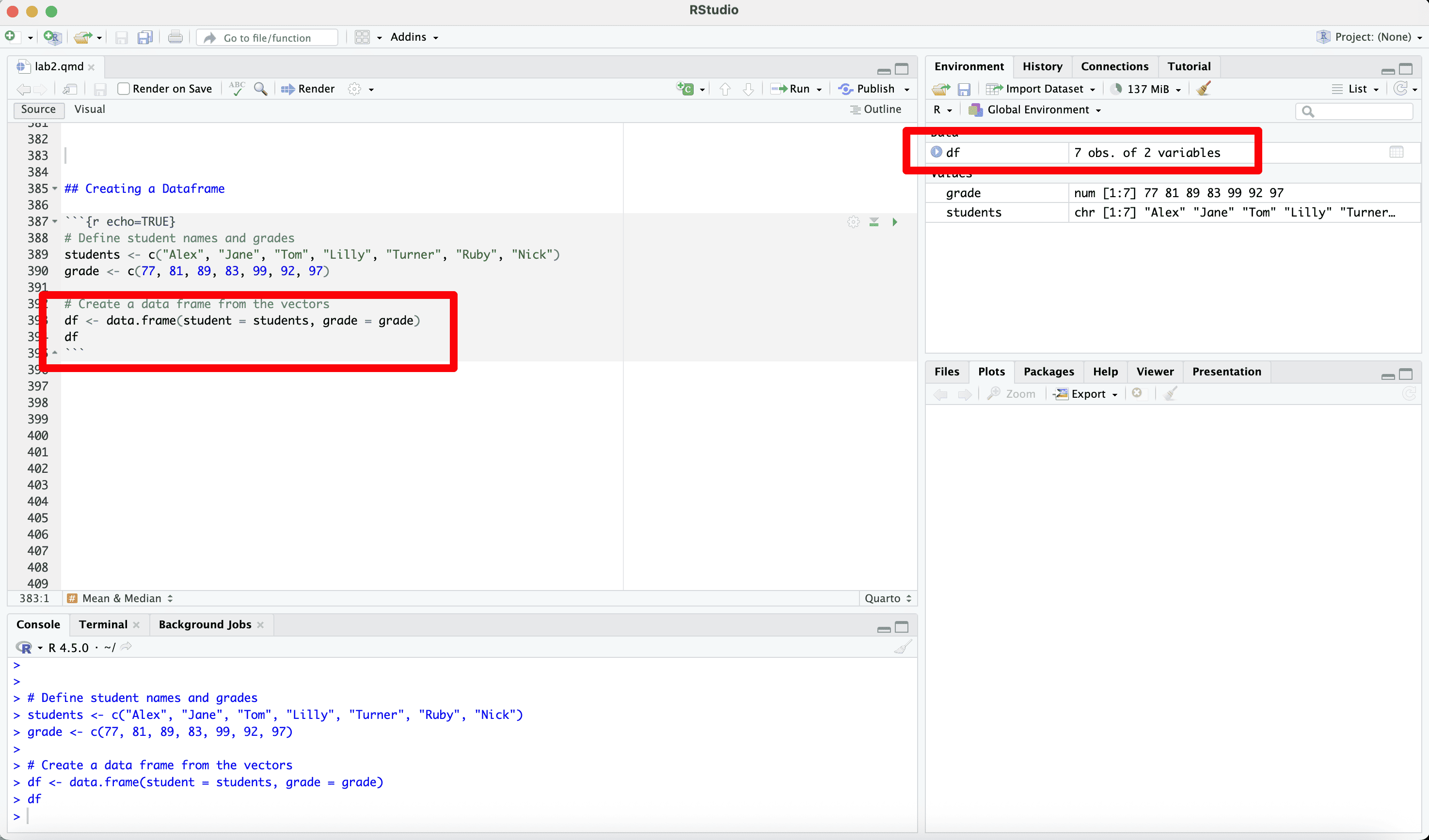
Creating a Dataframe
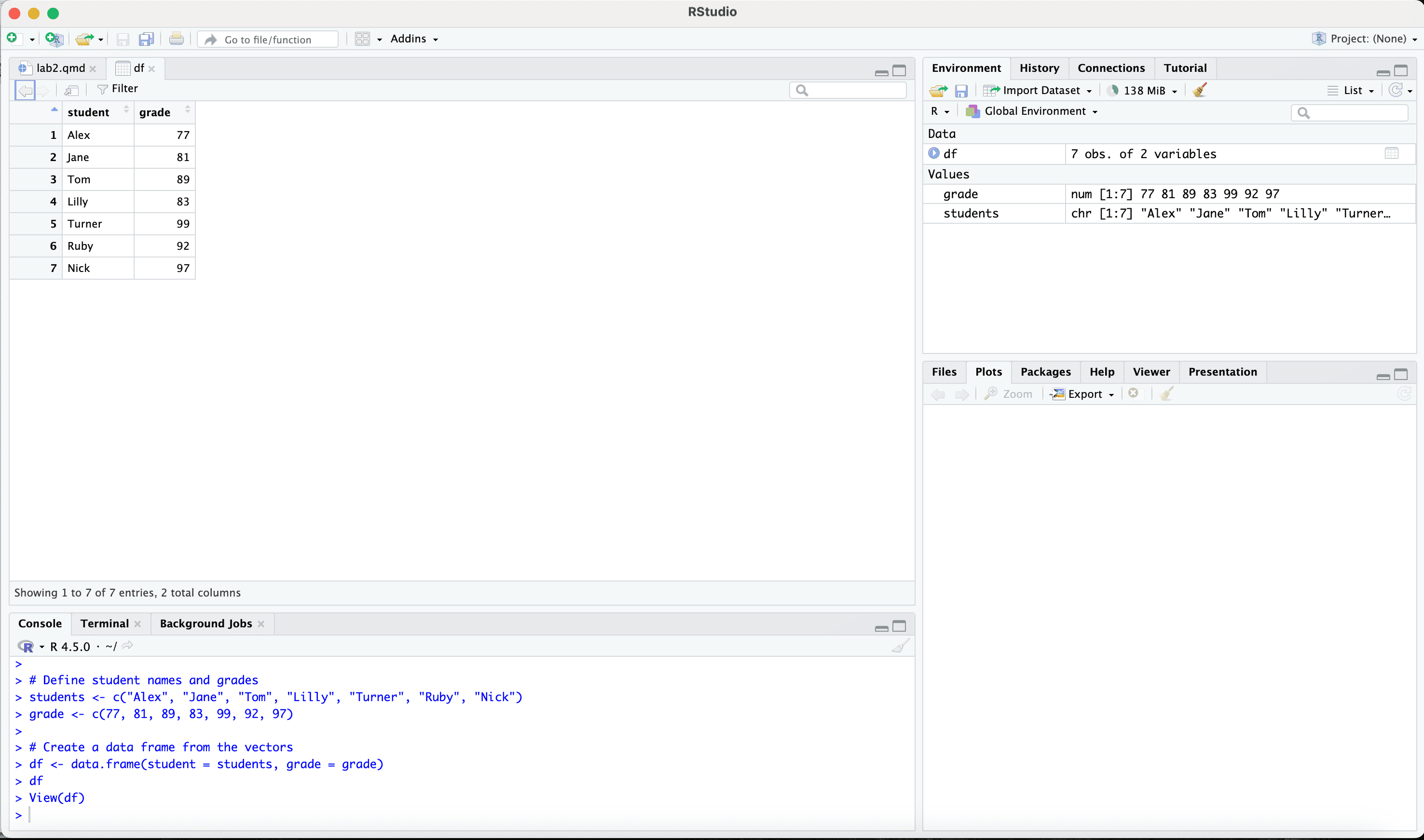
Creating a Dataframe
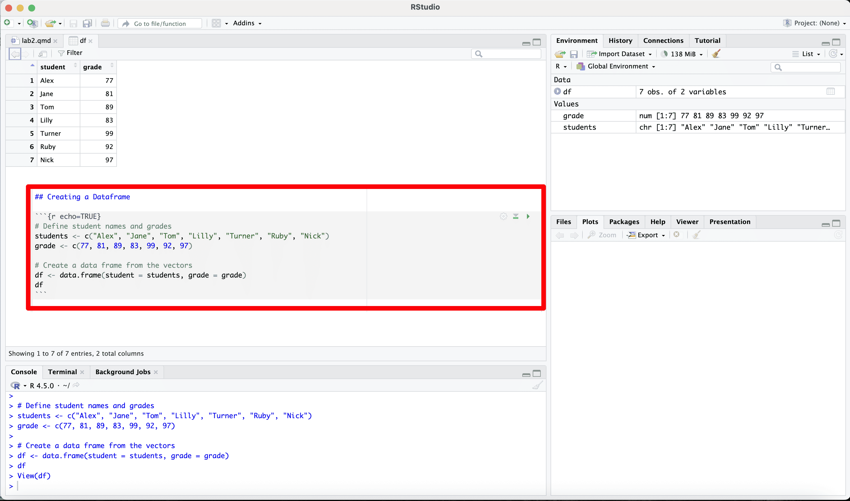
Creating a Dataframe
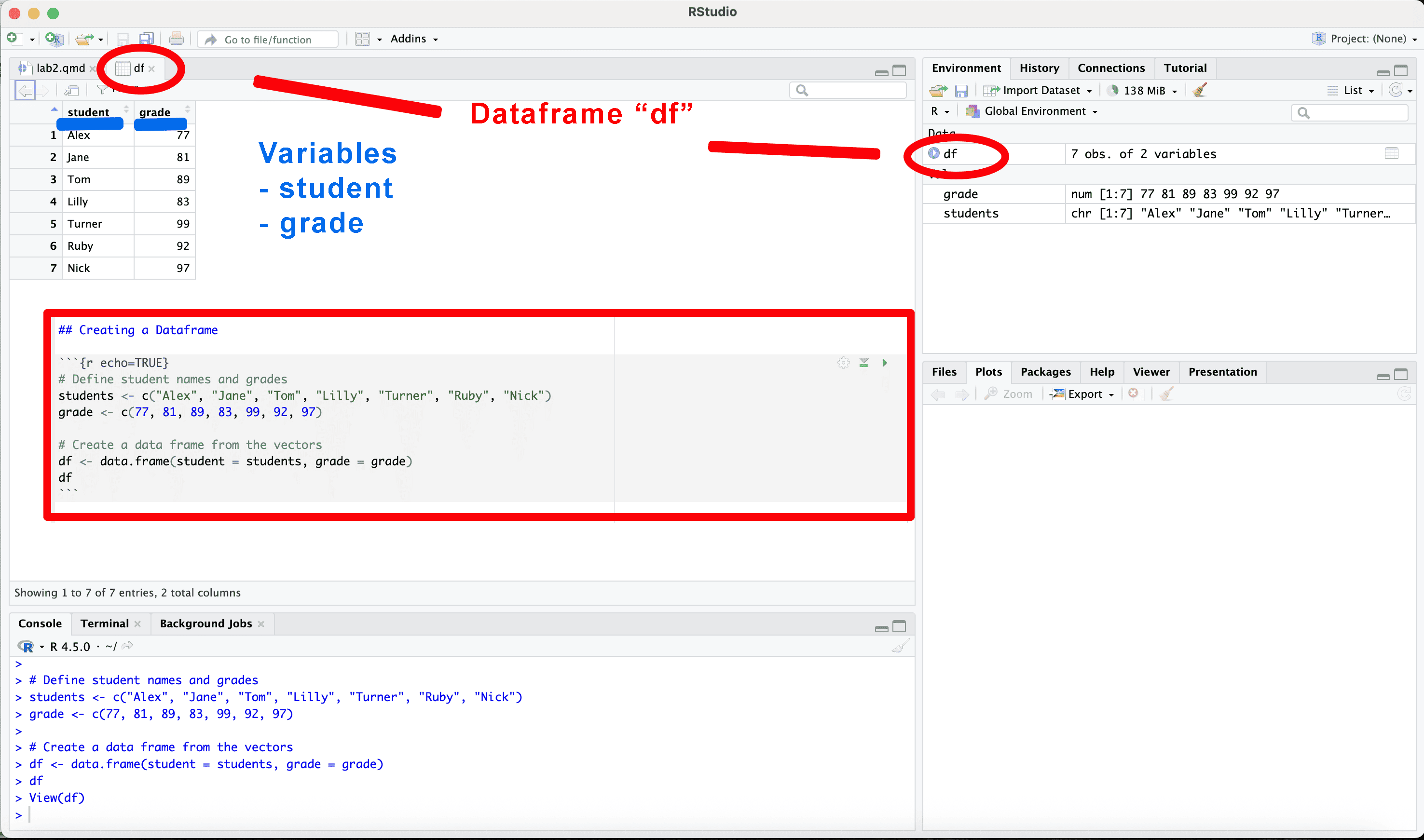
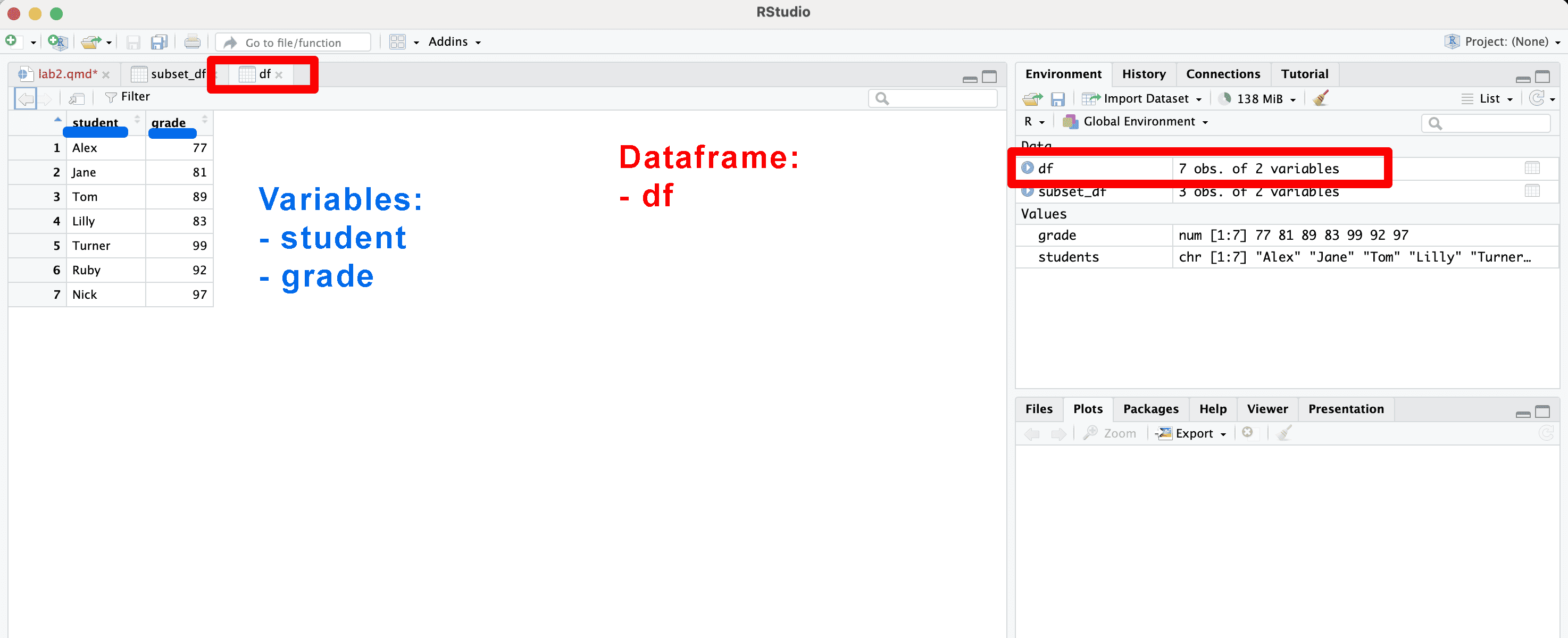
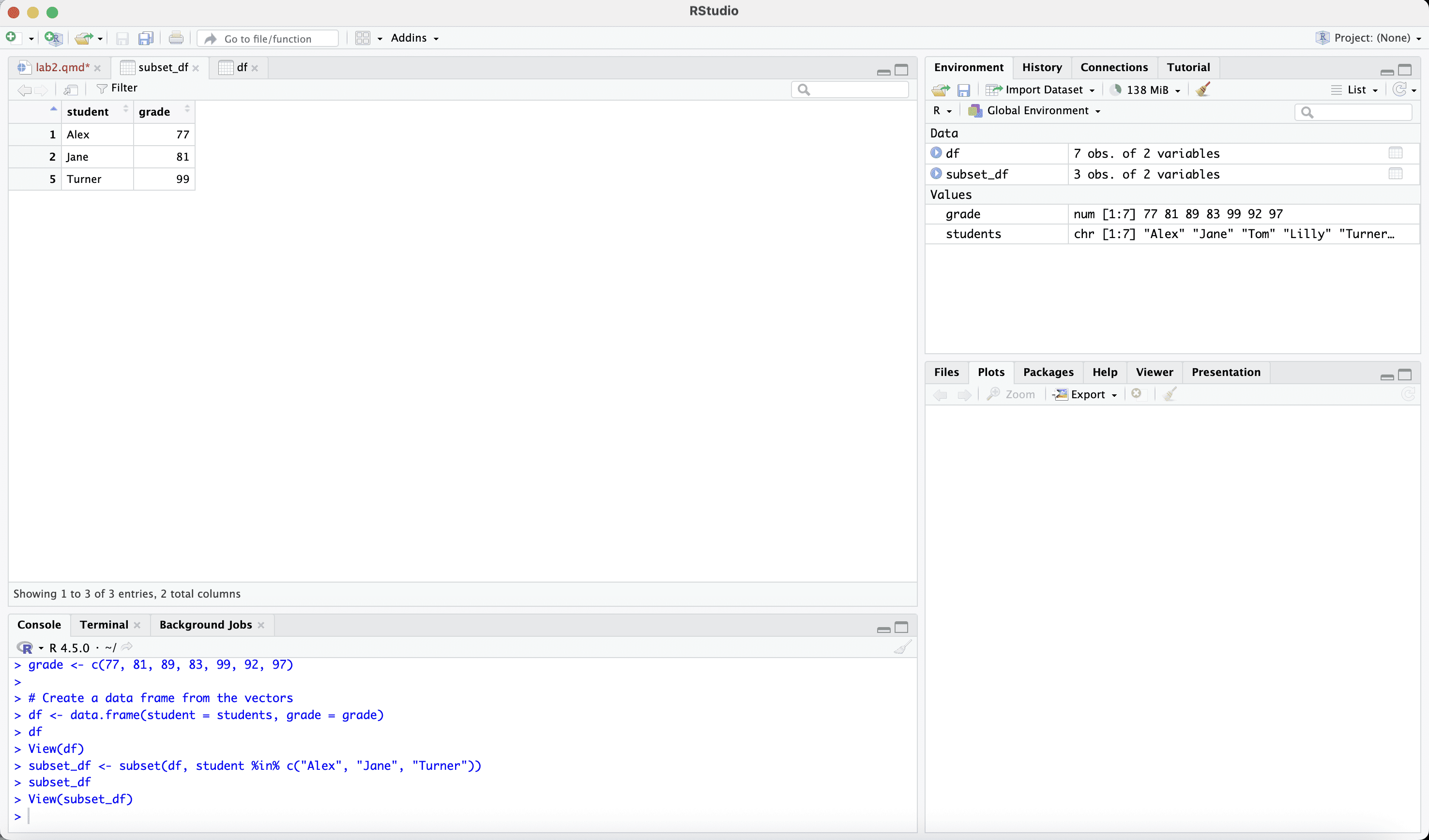
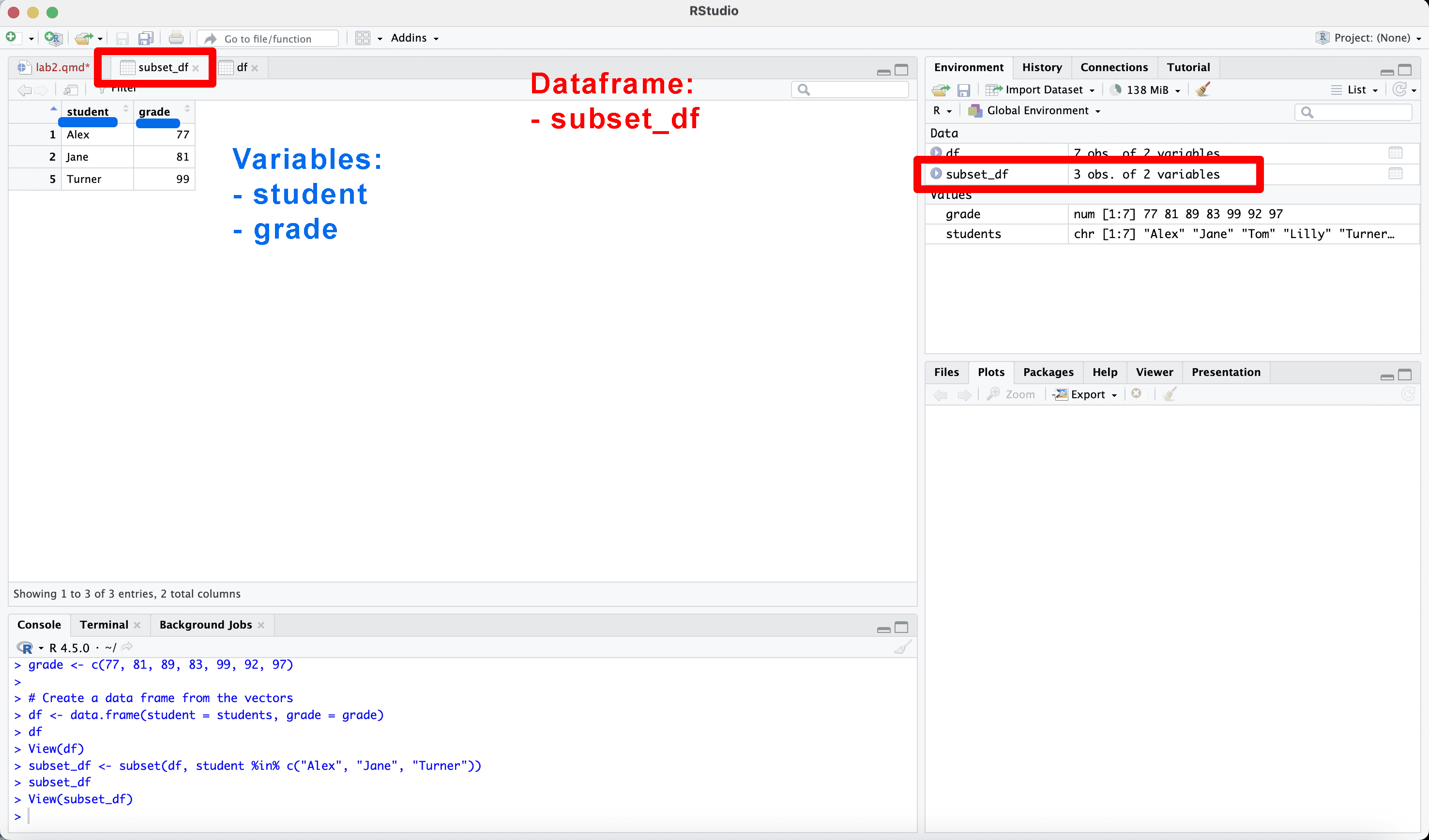
df is a dataframe
student and grade are variables within that dataframe
Creating a Dataframe

Creating a Dataframe
Creating a Dataframe
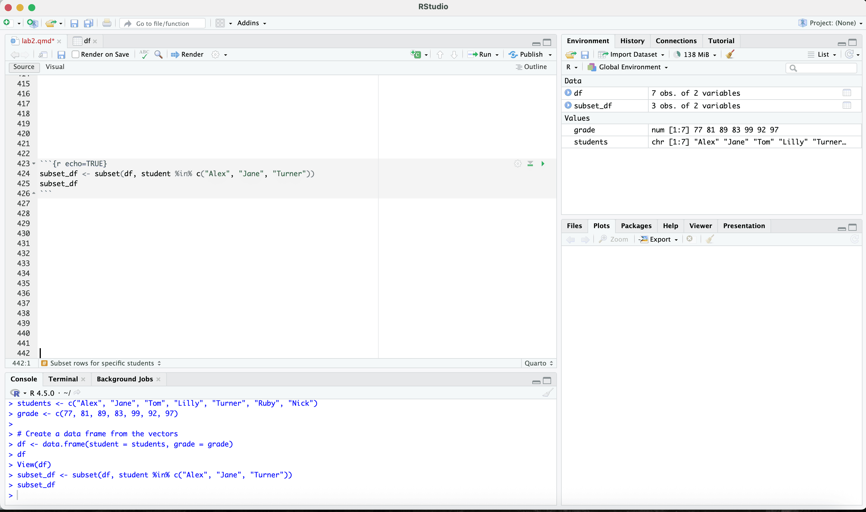
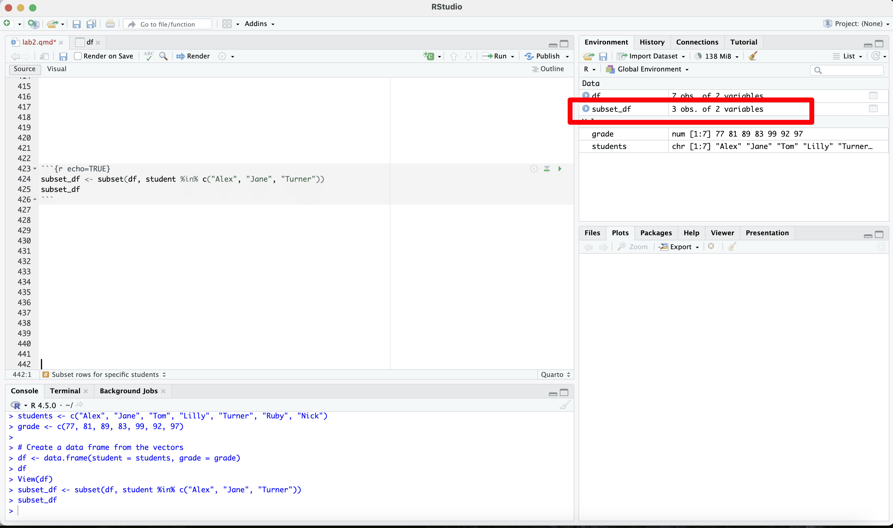
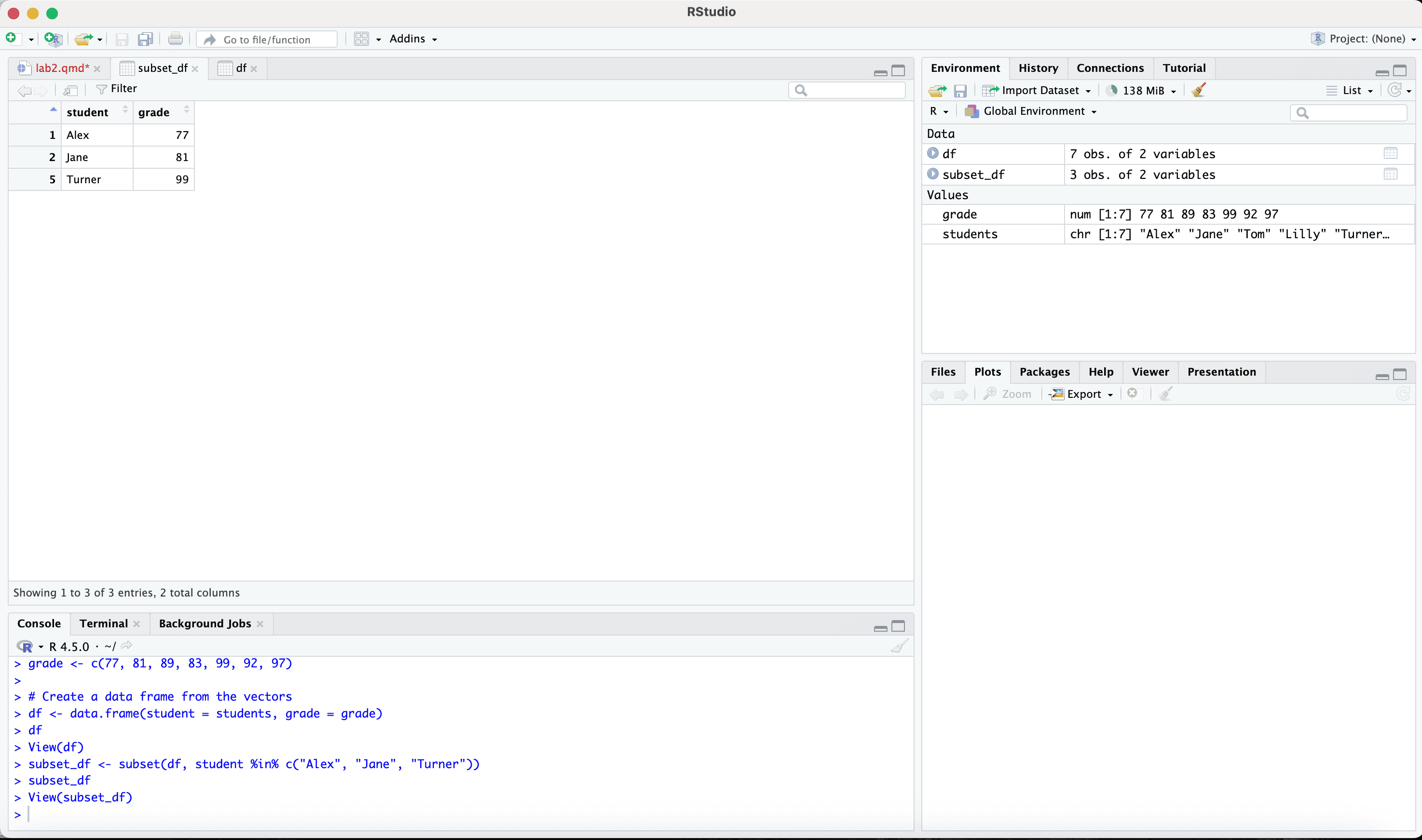
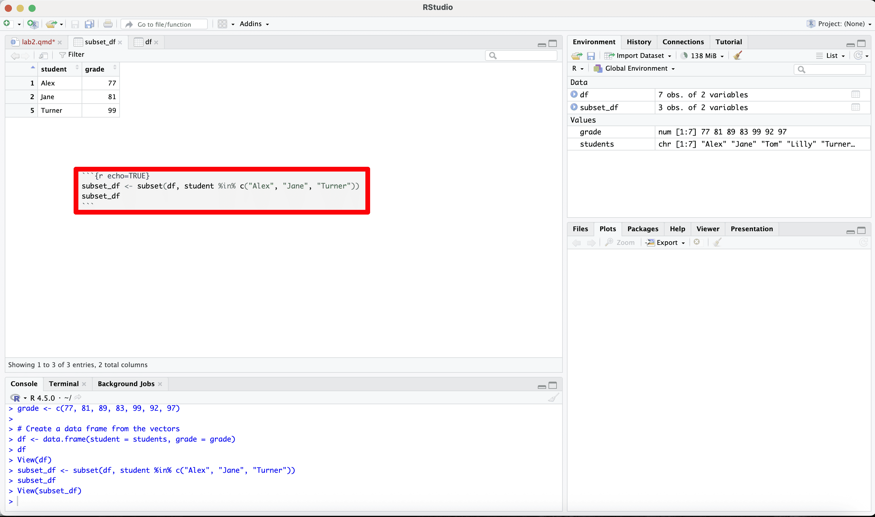
Subset rows for specific students
This is how we select specific observations
Creating a Dataframe
Subset rows for specific students
Creating a Dataframe
Subset rows for specific students
Creating a Dataframe
Subset rows for specific students
Creating a Dataframe
Subset rows for specific students
Summary Statistics
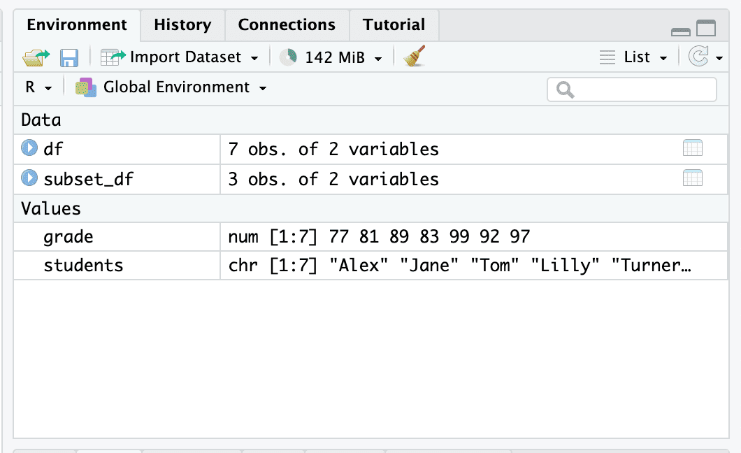
This is how we can calculate average for the two variables from the two dataframes
- Dataframe 1:
df - Dataframe 2:
subset_df
Summary Statistics
This is how we can calculate average for the two variables from the two dataframes
- Dataframe 1:
df - Dataframe 2:
subset_df
Summary Statistics
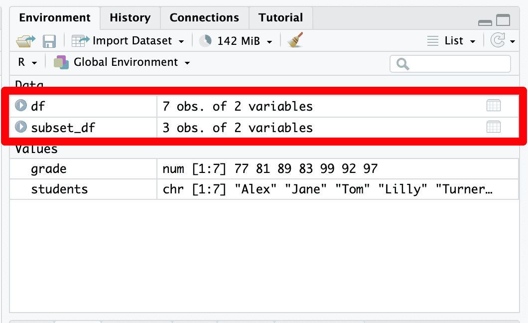
This is how we can calculate average for the two variables from the two dataframes
- Dataframe 1:
df - Dataframe 2:
subset_df
Summary Statistics
This is how we can calculate average for the two variables from the two dataframes
- Dataframe 1:
df - Dataframe 2:
subset_df
Summary Statistics
This is how we can calculate average for the two variables from the two dataframes
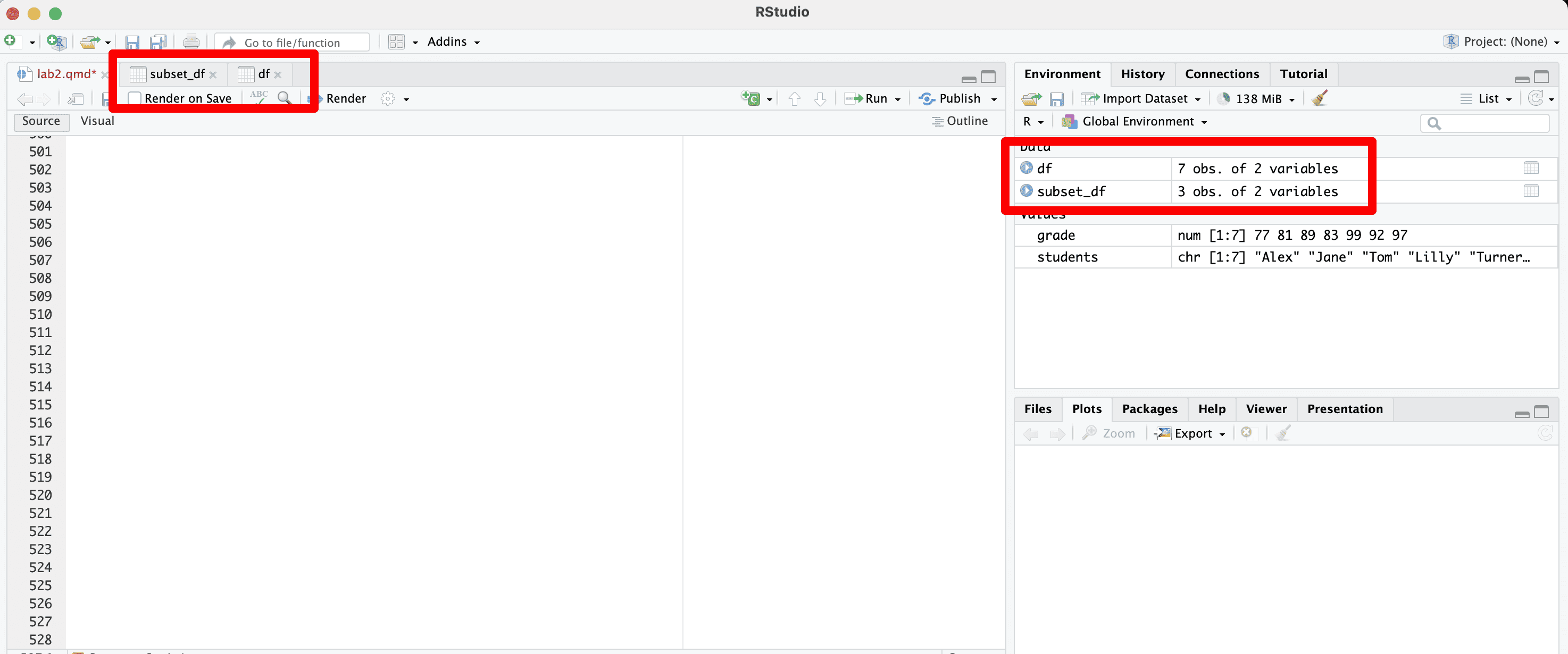
- Dataframe 1:
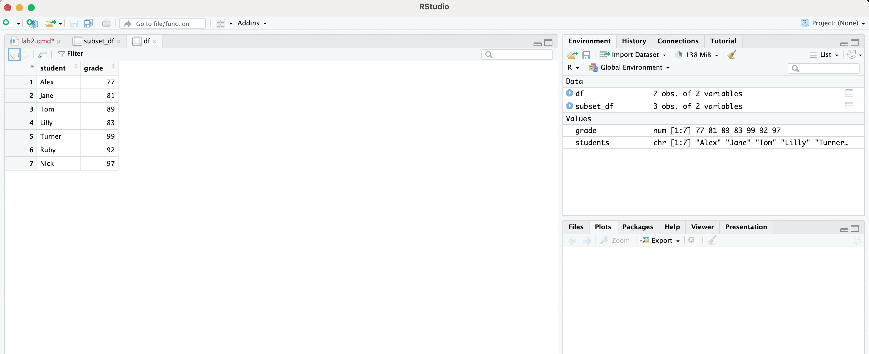
dfhas two variables:studentandgrade
Summary Statistics
Summary Statistics
Summary Statistics
This is how we can calculate average for the two variables from the two dataframes
- Dataframe 1:
dfhas two variables:studentandgrade
- Dataframe 2:
subset_dfhas two variables:studentandgrade
Summary Statistics
Summary Statistics
Summary Statistics
This is how we calculate the mean
Summary Statistics
This is how we identify Max & Min
Indexing Lists
This is how we work with indexing lists
Clearing Memory
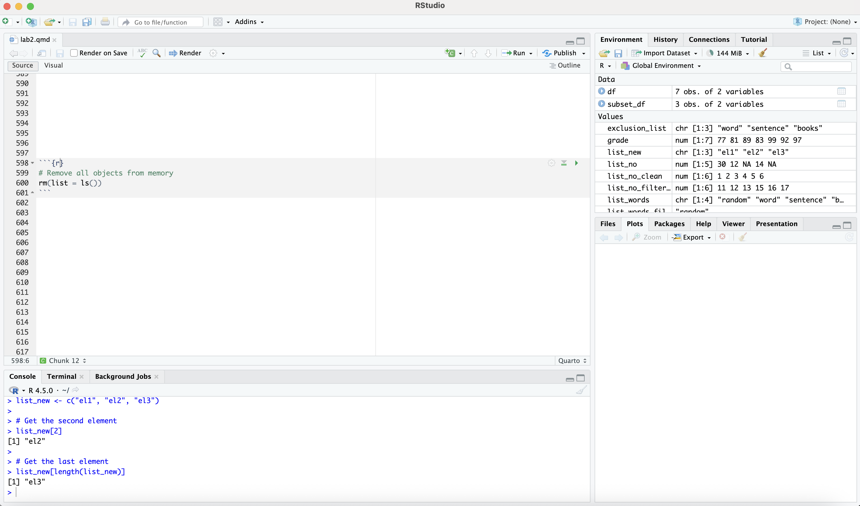
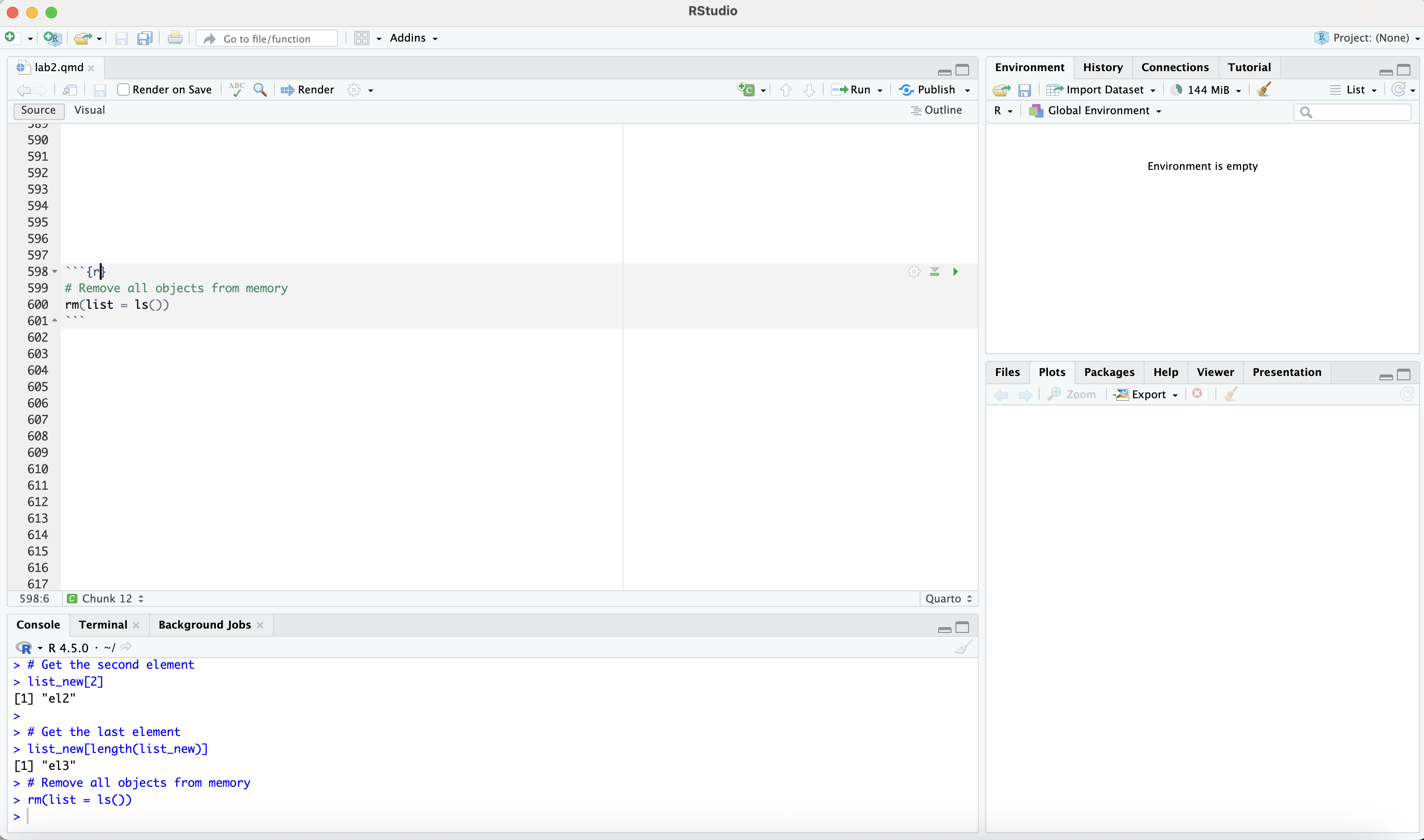
We can easily remove everything from your computer’s memory with the following command:
Clearing Memory
Notice the difference before and after
Clearing Memory
Notice the difference before and after
Loading External Datasets
Why Load External Files?
- Real-world data usually comes from external sources
- You’ll work with
.csv,.xlsx,.txt, or.tsvfiles
- Goal: Load the file → turn it into a data frame → analyze it
Loading External Datasets
Common File Types
| File Type | Description | R Function |
|---|---|---|
.csv |
Comma-separated values | read.csv() |
.tsv |
Tab-separated values | read.delim() |
.txt |
Generic text file | read.table() |
.xlsx |
Excel spreadsheet | readxl::read_excel() |
Opening a File
Download the following datasets from Dropbox:
Opening a File
Now put them in your working directory
Place it in a folder called “data” under the work directory (e.g. “week2/lab/” below)

Opening a File
To open the file add a new chunk and type
Opening a File
This is what you should see

Opening a File
This is what you should see

Opening a File
This is what you should see.
The part in red will differ from computer to computer

Opening a File
Notice how the path reflects your folder structure

Opening a File
Notice how the path reflects your folder structure

Opening a File
Notice how the path reflects your folder structure

Relative paths
We can now work with relative paths
Remember this?

Relative paths
We can now work with relative paths
Remember this?

Relative paths
We can now work with relative paths
Remember this?

Relative paths
We can now work with relative paths
Remember this?

Relative paths
We can now work with relative paths
Remember this?

Relative paths
This is how we read the csv file.
Relative paths
This is how we read the csv file.

Relative paths
We can now also load the other dataframe
Recap
Relative Paths vs. Absolute Paths
Notice the difference between relative paths vs. absolute paths
Relative Paths
Common Error
One common error is the following

Common Error
One common error is the following

Common Error
If you get that error, your path is not correct
Go back to the previous steps and identify the path to your file.
Our Data
Let us now investigate our two datasets
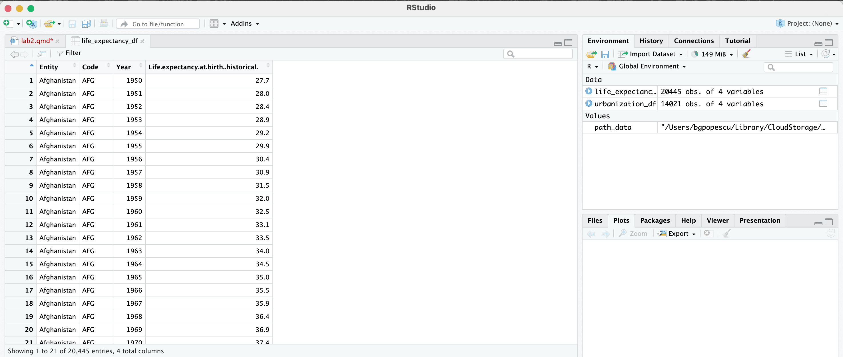
Our Data
Let us now investigate our two datasets
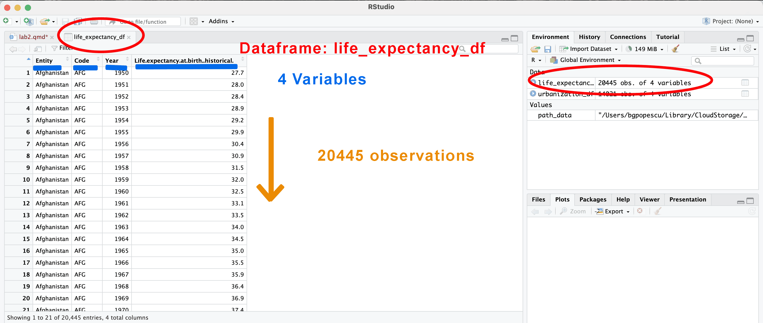
Our Data
Let us now investigate our two datasets
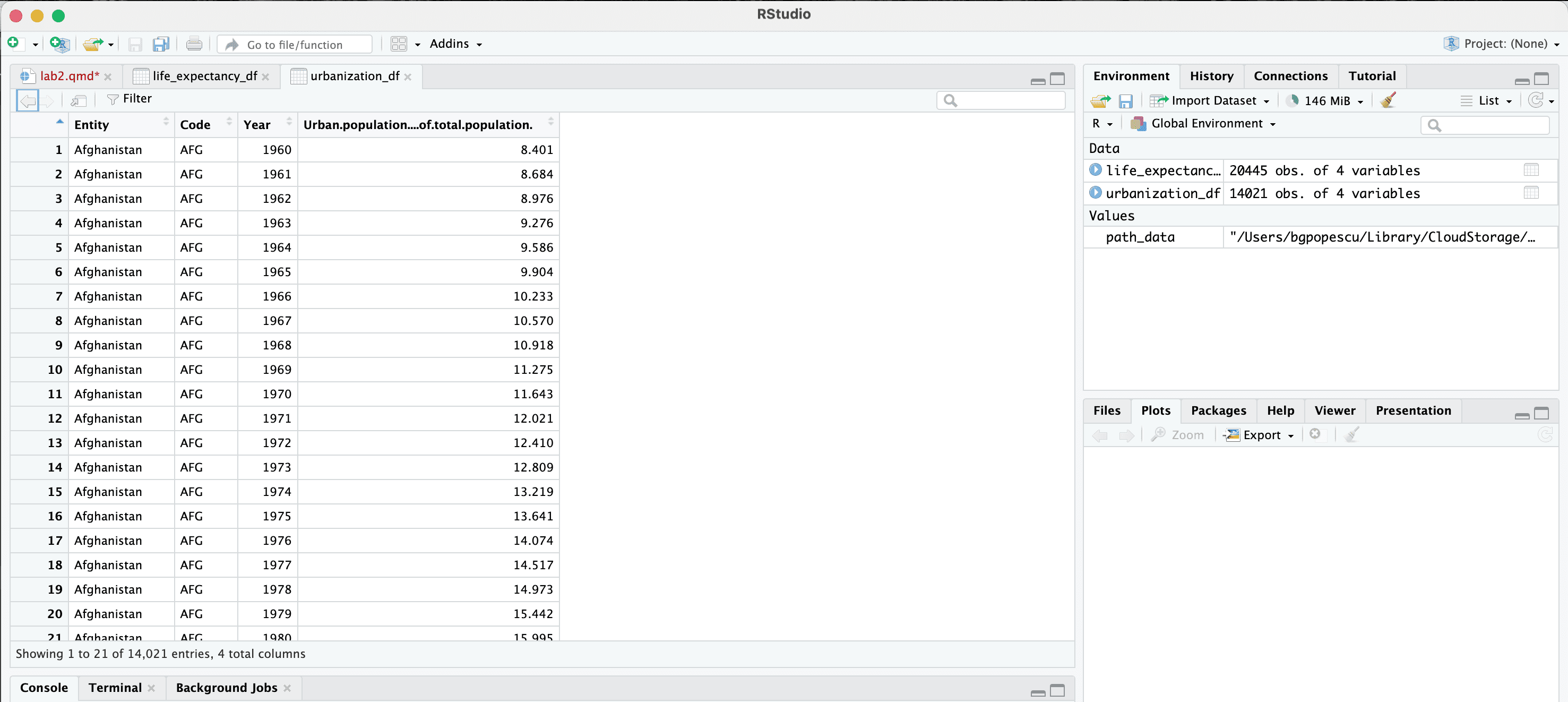
Our Data
Let us now investigate our two datasets
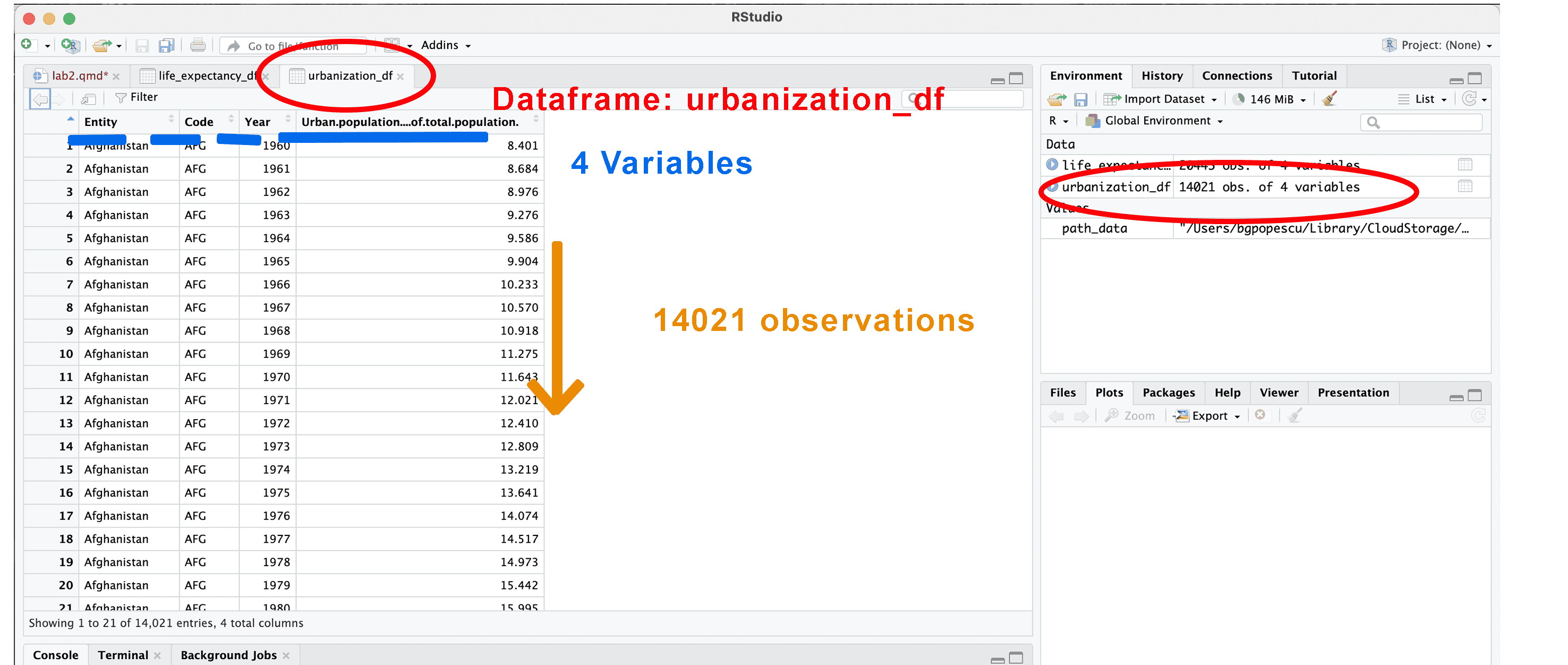
Our Data
Examining the First Entries
This is how we can examine the first five entries
You should see:
Our Data
Examining the First Entries
This is how we can examine the first five entries
You should see:
Installing Packages
This is how you install a packages in R
Notice that you need to have quotes: "tidyverse"
Once you are done:
- delete
install.packages("tidyverse") - or comment it out by adding “#”
If you don’t delete it or comment it out, it will cause errors during rendering.
Once you install the package, it will always be on your machine.
Installing Packages
Errors
As we progress, you might be using commands, that might result in:
Installing Packages
Loading Packages
To use the commands associated with the package, you need to load it
You will need to load this package to use its functions
Our Data
Examining the First Entries using glimpse
We will examine our data using glimpse
Rows: 20,445
Columns: 4
$ Entity                                <chr> "Afghanistan", "Afghanistan", "A…
$ Code                                  <chr> "AFG", "AFG", "AFG", "AFG", "AFG…
$ Year                                  <int> 1950, 1951, 1952, 1953, 1954, 19…
$ Life.expectancy.at.birth..historical. <dbl> 27.7, 28.0, 28.4, 28.9, 29.2, 29…
or
Rows: 20,445
Columns: 4
$ Entity                                <chr> "Afghanistan", "Afghanistan", "A…
$ Code                                  <chr> "AFG", "AFG", "AFG", "AFG", "AFG…
$ Year                                  <int> 1950, 1951, 1952, 1953, 1954, 19…
$ Life.expectancy.at.birth..historical. <dbl> 27.7, 28.0, 28.4, 28.9, 29.2, 29…
Our Data
Examining the First Entries using glimpse
We will examine our data using glimpse
Rows: 20,445
Columns: 4
$ Entity                                <chr> "Afghanistan", "Afghanistan", "A…
$ Code                                  <chr> "AFG", "AFG", "AFG", "AFG", "AFG…
$ Year                                  <int> 1950, 1951, 1952, 1953, 1954, 19…
$ Life.expectancy.at.birth..historical. <dbl> 27.7, 28.0, 28.4, 28.9, 29.2, 29…
We have four variables within our dataframe:
Entity: string or character variableCode: string or character variableYear: numeric or integer variableLife.expectancy.at.birth..historical.: numeric or double precision variable
Our Data
Examining the First Entries using glimpse
We will examine our data using glimpse
Rows: 20,445
Columns: 4
$ Entity                                <chr> "Afghanistan", "Afghanistan", "A…
$ Code                                  <chr> "AFG", "AFG", "AFG", "AFG", "AFG…
$ Year                                  <int> 1950, 1951, 1952, 1953, 1954, 19…
$ Life.expectancy.at.birth..historical. <dbl> 27.7, 28.0, 28.4, 28.9, 29.2, 29…
We have four variables within our dataframe:
Entity: the country: “Afghanistan”, “Albania”, “Algeria”, etc.Code: the country code: “AFG”, “ALB”, “DZA”, etcYear: year 1950, 1951, 1952, etc.Life.expectancy.at.birth..historical.: life expectancy corresponding to that year
We Learned a Few Things Today
- Creating and Subsetting Dataframe
- Loading External files:
.csvand.xlsx - Relative vs. Absolute Paths
- Handling file or directory errors
- Examining entries in a dataframe
Popescu (JCU): Dataframes, Lists, External Files, Paths