L14: Spatial Operations

Open Street Maps (OSM), Coordinate Systems, Buffers, Intersections, Unions

Bogdan G. Popescu

bogdan.popescu@johncabot.edu

John Cabot University

GIS Operations

1. Open Street Maps
2. Polygon Centroid
3. Changing Coordinate Systems
4. Creating Buffers
5. Uniting different shapes in one
6. Intersections
7. Unions

Open Street Maps

Open Street Maps or OSM is a collaborative mapping project established in 2004.

Open Street Maps

• OSM is a great resource for open, rights-free geographic data.

• However, data coverage and quality varies

  • Rich countries/areas have better coverage
  • Rich countries/areas have better quality

• Ideally, you should still aim to use reliable data from governments or other sources

Open Street Maps

• Data in OSM is saved under different geometry types

• Points
• Lines
• Polygons

• The tags within these geometries describe the attributes of the features shown

• A very useful guide for how to use OSM can be found at: https://wiki.openstreetmap.org

• Similarly, the following guide explains how to extract data from Open Street Maps: https://wiki.openstreetmap.org/wiki/Downloading_data

OSM and Geofabrik

Using OSM data can prove cumbersome

One alternative is to use OSM pre-processed data

One good source for pre-processed OSM data is: http://www.geofabrik.de

Agenda for Today

In this class we will use OSM data to deal with a hypothetical scenario.

Let’s assume that we represent a consulting company in Rome that helps international students find suitable accommodation in Rome

Within this hypothetical scenario, we will use a series of GIS operations:

• calculating polygon centroids
• changing coordinate systems
• creating buffers
• uniting different shapes in one
• intersecting shapes
• creating unions of overlapping shapefiles

Scenario

Imagine the following hypothetical scenario

Mark is an exchange student from the US and he will be at JCU for a whole year.

Here are Mark’s specifications for the ideal apartment:

• living 1.5km (0.93 miles) away from JCU.

• living 0.7km (0.43 miles) away from the Vatican.

• living 0.5km (0.31 miles) from a bank.

This is very interesting realistic scenario.

Identifying JCU on the Rome Map

Step 1: Let’s first identify where JCU is

Buffers

Buffers are polygons around input features to a specified distance.

Buffers

Buffers are polygons around input features to a specified distance.

Buffers

Buffers are polygons around input features to a specified distance.

Buffers

Buffers are polygons around input features to a specified distance.

Buffers

Buffers are polygons around input features to a specified distance.

Buffers

Buffers are polygons around input features to a specified distance.

Buffers

Buffers are polygons around input features to a specified distance.

Buffers

Buffers are polygons around input features to a specified distance.

Buffers

Buffers are polygons around input features to a specified distance.

Creating the 1500 m buffer

Step 2: Let’s create the 1500m buffer around JCU

Creating the 1500 m buffer

Step 2: Let’s create the 1500m buffer around JCU

Including the Vatican

Including the Vatican 700m buffer

Including the banks

Including the banks 500m buffer

Including all the buffers

Intersecting all Buffers and Taking the Union

Zooming into the Common Area

This is the area that fits Mark’s requirements:

• living 1.5km (0.93 miles) away from JCU.
• living 0.7km (0.43 miles) away from the Vatican.
• living 0.5km (0.31 miles) from a bank.

What are the actual steps?

• Step1: Download the relevant shapefiles

• Step2: Map the data

• Step3: Identify JCU

• Step4: Change the coordinate system of the JCU metric system

• Step5: Create the buffer of 1500m around the university

• Step6: Change the coordinate system back to degrees

• Step7: Map the buffer

• Step8: Repeat the procedures for the other units (Vatican and banks)

What are the actual steps?

• Step9: Intersect the Buffers

• Step10: Identify the common area

Step1: Download the relevant shapefiles

A great datasource for urban data is Open Street Maps (OSM)

However downloading all that data can be difficult

One way to make that data more manageable is to download data from: http://download.geofabrik.de

Geofabrik extract, select, and process free geodata for you on a regular basis, for free.

Step1: Download the relevant shapefiles

Step1: Download the relevant shapefiles

Step1: Download the relevant shapefiles

Step1: Download the relevant shapefiles

Step1: Download the relevant shapefiles

Step1: Download the relevant shapefiles

Step1: Download the relevant shapefiles

Step1: Download the relevant shapefiles

Step1: Download the relevant shapefiles

Step1: Download the relevant shapefiles

In the interest of time you can download the shapefiles that I prepared.

The geodatabase can be downloaded from:

• OSM Rome selection

Unzip the file and place it a folder called “data” within the relevant week.

Step2: Loading the data

library(sf)
library(ggplot2)
gis_buildings <- st_read(dsn="./data/selection.gdb",
                         layer="gis_osm_buildings", quiet = T)

gis_osm_roads <- st_read(dsn="./data/selection.gdb",
                         layer="gis_osm_roads", quiet = T)

gis_osm_pofw <- st_read(dsn="./data/selection.gdb", 
                         layer="gis_osm_pofw", quiet = T)

gis_osm_pois <- st_read(dsn="./data/selection.gdb", 
                         layer="gis_osm_pois", quiet = T)

Step2: Loading the data

fig1<-ggplot()+
  geom_sf(data=gis_buildings, fill="grey")+
  geom_sf(data=gis_osm_roads, linewidth = 0.1, color = "red", alpha=0.5)
fig1

Step3: Identify Relevant Points of Interest

This is all the data

We want to zoom into JCU.

Step3: Identify Relevant Points of Interest

This is all the data.

We want to zoom into JCU. Before we do that, we need to find JCU.

Step3: Identify Relevant Points of Interest

To identify the points of interest, we simply go to the dataframe and try to identify them

Step3: Identify Relevant Points of Interest

To identify the points of interest we simply go to the dataframe and try to identify them

Step3: Identify Relevant Points of Interest

To identify the points of interest we simply go to the dataframe and try to identify them

Step3: Identify Relevant Points of Interest

To identify the points of interest we simply go to the dataframe and try to identify them

Step3: Identify Relevant Points of Interest

To identify the points of interest we simply go to the dataframe and try to identify them

Step3: Identify Relevant Points of Interest

To identify the points of interest we simply go to the dataframe and try to identify them

Step3: Identify Relevant Points of Interest

To identify the points of interest we simply go to the dataframe and try to identify them

Step3: Identify Relevant Points of Interest

To identify the points of interest we simply go to the dataframe and try to identify them

Step3: Identify Relevant Points of Interest

We can now create sepaeate dataframe:

jcu <- subset(gis_buildings, name=="John Cabot University - Tiber Campus")
glimpse(jcu)

Rows: 1
Columns: 8
$ osm_id       <chr> "203509198"
$ code         <int> 1500
$ fclass       <chr> "building"
$ name         <chr> "John Cabot University - Tiber Campus"
$ type         <chr> " "
$ Shape_Length <dbl> 0.001311444
$ Shape_Area   <dbl> 7.82957e-08
$ Shape        <MULTIPOLYGON [°]> MULTIPOLYGON (((12.47205 41...

Step3: Identify Relevant Points of Interest

We can now create separate dataframe:

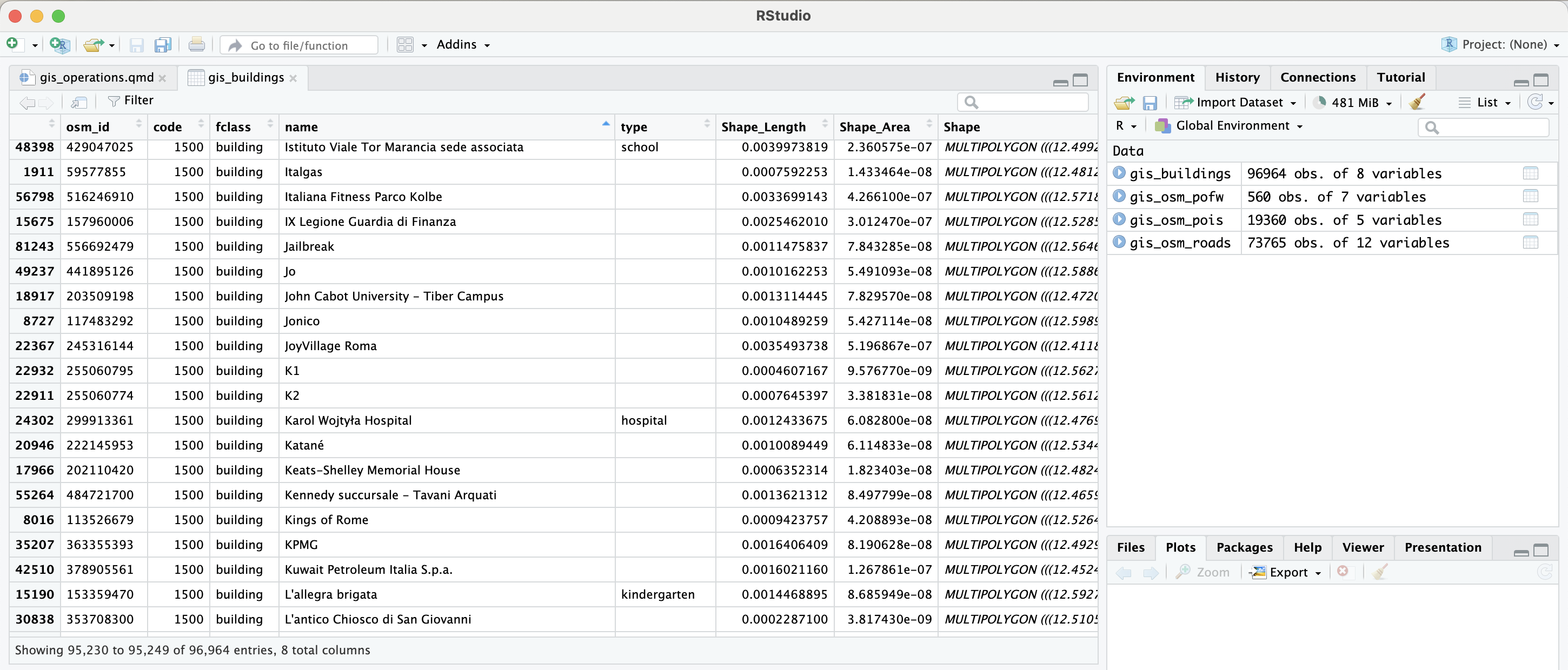
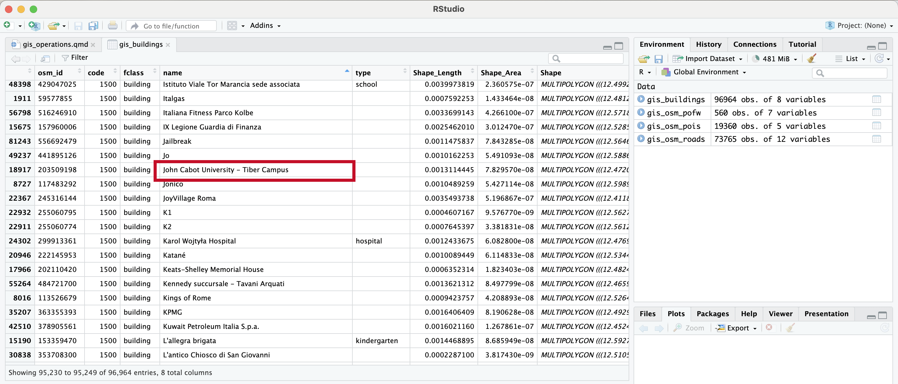
jcu <- subset(gis_buildings, name=="John Cabot University - Tiber Campus")

So, this is now a separate dataframe with one observation.

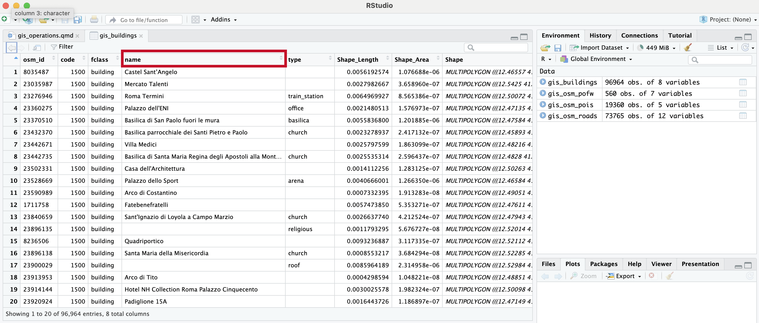
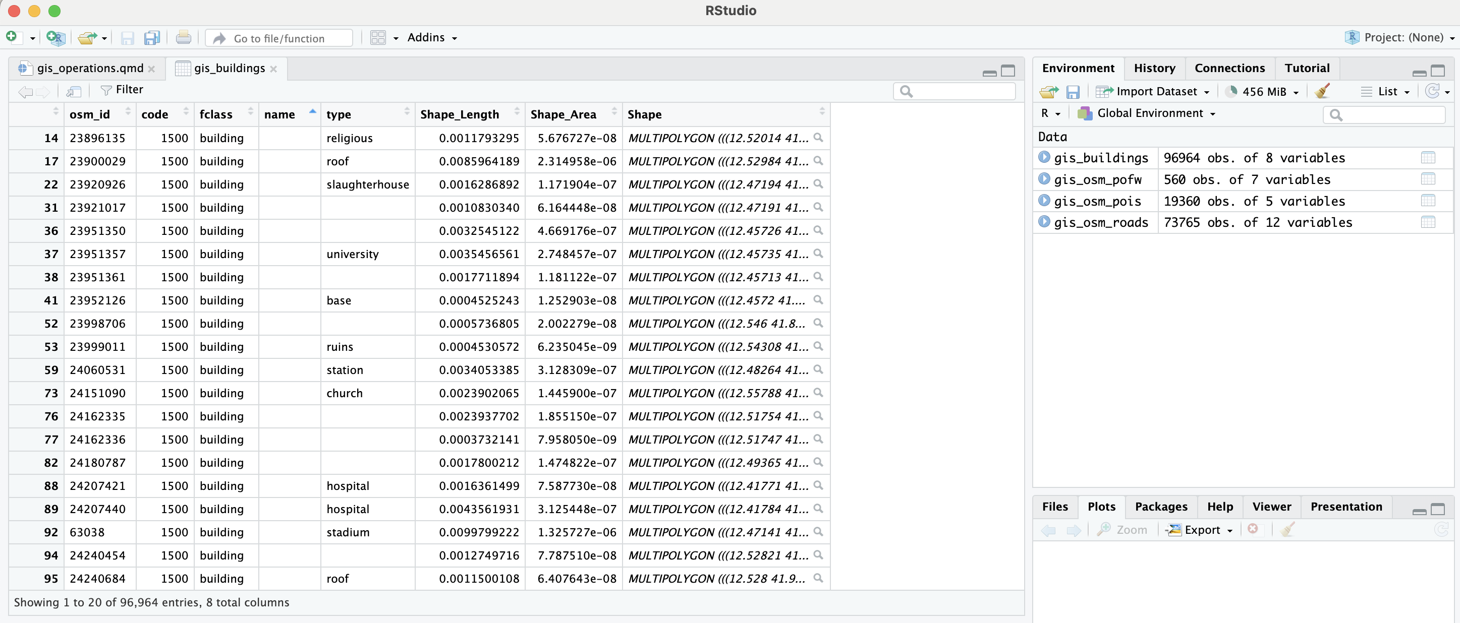
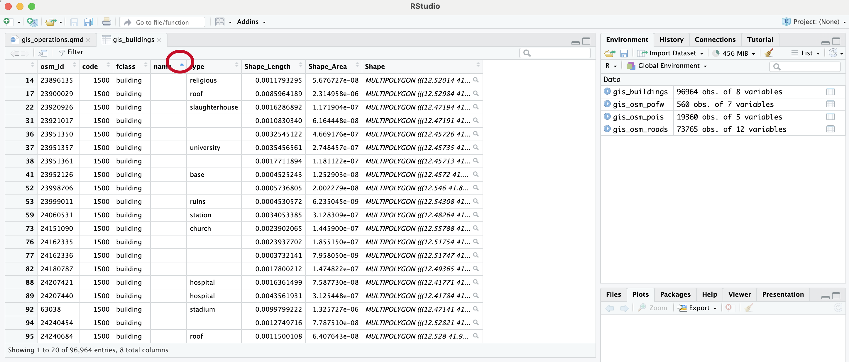
Step3: Identify Relevant Points of Interest

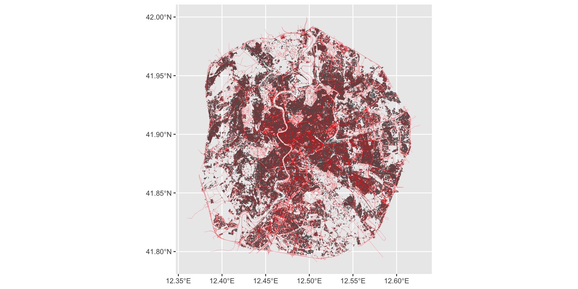
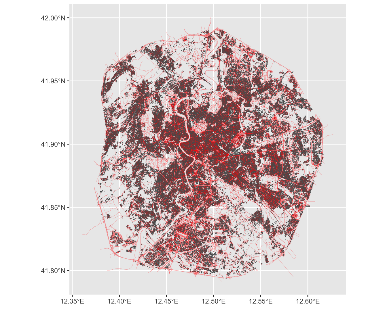
We can map it on top of all the other files

fig2<-ggplot()+
  geom_sf(data=gis_buildings, fill="grey")+
  geom_sf(data=gis_osm_roads, linewidth = 0.1, color = "red", alpha=0.5)+
  geom_sf(data=jcu, linewidth = 0.1, color = "green", fill = "green", alpha=0.5)
fig2

Step3: Identify Relevant Points of Interest

We can map it on top of all the other files.

JCU is barely visible. We therefore have to zoom in

Step3: Identify Relevant Points of Interest

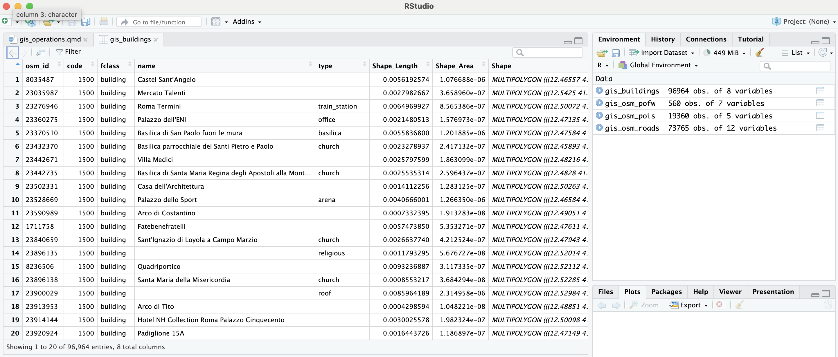
To zoom in, we need to find JCU’s coordinates

#Examining the object
jcu

Simple feature collection with 1 feature and 7 fields
Geometry type: MULTIPOLYGON
Dimension:     XY
Bounding box:  xmin: 12.47205 ymin: 41.89028 xmax: 12.47249 ymax: 41.89061
Geodetic CRS:  WGS 84
         osm_id code   fclass                                 name type
18917 203509198 1500 building John Cabot University - Tiber Campus     
      Shape_Length  Shape_Area                          Shape
18917  0.001311444 7.82957e-08 MULTIPOLYGON (((12.47205 41...

Step3: Identify Relevant Points of Interest

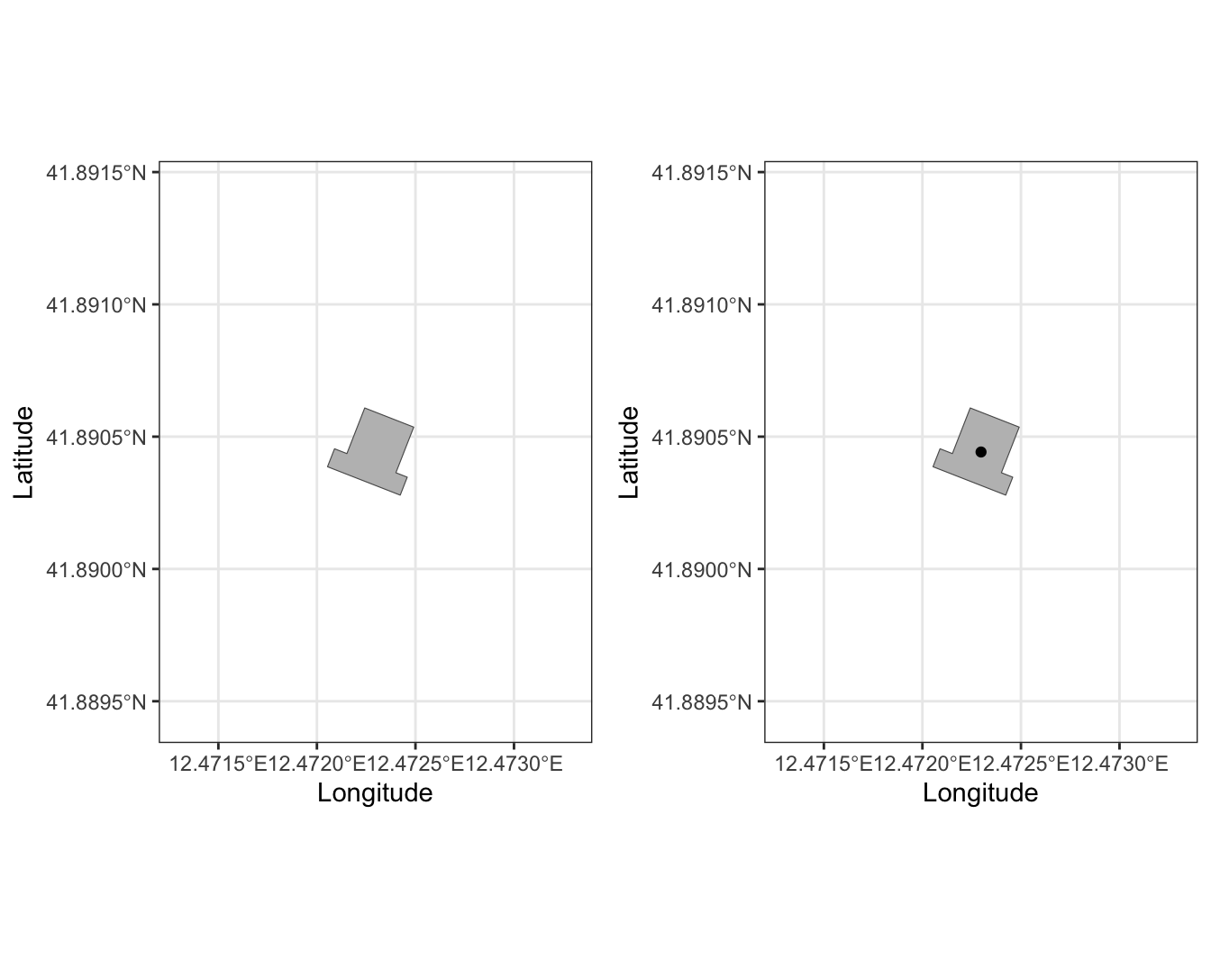
Finding the centroid of the JCU polygon

#Calling out the geometry of the object
st_geometry(jcu)

Geometry set for 1 feature 
Geometry type: MULTIPOLYGON
Dimension:     XY
Bounding box:  xmin: 12.47205 ymin: 41.89028 xmax: 12.47249 ymax: 41.89061
Geodetic CRS:  WGS 84

Step3: Identify Relevant Points of Interest

Finding the centroid of the JCU polygon

#Identifying the centroid of the geometry of the object
st_centroid(st_geometry(jcu))

Geometry set for 1 feature 
Geometry type: POINT
Dimension:     XY
Bounding box:  xmin: 12.4723 ymin: 41.89044 xmax: 12.4723 ymax: 41.89044
Geodetic CRS:  WGS 84

Step3: Identify Relevant Points of Interest

Finding the centroid of the JCU polygon

#Saving the lat lon of the centroid of the geometry of the object and adding it as a separate field
jcu$lonlat<-st_centroid(st_geometry(jcu))
jcu

Simple feature collection with 1 feature and 7 fields
Active geometry column: Shape
Geometry type: MULTIPOLYGON
Dimension:     XY
Bounding box:  xmin: 12.47205 ymin: 41.89028 xmax: 12.47249 ymax: 41.89061
Geodetic CRS:  WGS 84
         osm_id code   fclass                                 name type
18917 203509198 1500 building John Cabot University - Tiber Campus     
      Shape_Length  Shape_Area                          Shape
18917  0.001311444 7.82957e-08 MULTIPOLYGON (((12.47205 41...
                        lonlat
18917 POINT (12.4723 41.89044)

Step3: Identify Relevant Points of Interest

Finding the centroid of the JCU polygon

#Splitting the lat lon into two different columns
jcu[c('lon_x', 'lat_y')]<-str_split_fixed(jcu$lonlat, ",", 2)
jcu

Simple feature collection with 1 feature and 9 fields
Active geometry column: Shape
Geometry type: MULTIPOLYGON
Dimension:     XY
Bounding box:  xmin: 12.47205 ymin: 41.89028 xmax: 12.47249 ymax: 41.89061
Geodetic CRS:  WGS 84
         osm_id code   fclass                                 name type
18917 203509198 1500 building John Cabot University - Tiber Campus     
      Shape_Length  Shape_Area                          Shape
18917  0.001311444 7.82957e-08 MULTIPOLYGON (((12.47205 41...
                        lonlat              lon_x              lat_y
18917 POINT (12.4723 41.89044) c(12.4722974446979  41.8904420317772)

Step3: Identify Relevant Points of Interest

Finding the centroid of the JCU polygon

#Removing "c(" from "c(12.4722974446979" and "(" from "41.8904420317772)"
jcu$lon_x<-str_replace(jcu$lon_x, "c\\(", "")
jcu$lat_y<-str_replace(jcu$lat_y, "\\)", "")
jcu

Simple feature collection with 1 feature and 9 fields
Active geometry column: Shape
Geometry type: MULTIPOLYGON
Dimension:     XY
Bounding box:  xmin: 12.47205 ymin: 41.89028 xmax: 12.47249 ymax: 41.89061
Geodetic CRS:  WGS 84
         osm_id code   fclass                                 name type
18917 203509198 1500 building John Cabot University - Tiber Campus     
      Shape_Length  Shape_Area                          Shape
18917  0.001311444 7.82957e-08 MULTIPOLYGON (((12.47205 41...
                        lonlat            lon_x             lat_y
18917 POINT (12.4723 41.89044) 12.4722974446979  41.8904420317772

Step3: Identify Relevant Points of Interest

Finding the centroid of the JCU polygon

#Making lon_x and lat_y numeric (they are strings)
jcu$lon_x<-as.numeric(jcu$lon_x)
jcu$lat_y<-as.numeric(jcu$lat_y)
jcu

Simple feature collection with 1 feature and 9 fields
Active geometry column: Shape
Geometry type: MULTIPOLYGON
Dimension:     XY
Bounding box:  xmin: 12.47205 ymin: 41.89028 xmax: 12.47249 ymax: 41.89061
Geodetic CRS:  WGS 84
         osm_id code   fclass                                 name type
18917 203509198 1500 building John Cabot University - Tiber Campus     
      Shape_Length  Shape_Area                          Shape
18917  0.001311444 7.82957e-08 MULTIPOLYGON (((12.47205 41...
                        lonlat   lon_x    lat_y
18917 POINT (12.4723 41.89044) 12.4723 41.89044

Step3: Identify Relevant Points of Interest

Finding the centroid of the JCU polygon

We can now identify the min and max lon and lat for our map.

These will allow us to decide how much we should zoom in or zoom out.

min_lon_x<-min(jcu$lon_x)
min_lon_x

[1] 12.4723

Step3: Identify Relevant Points of Interest

Finding the centroid of the JCU polygon

We can now identify the min and max lon and lat for our map.

These will allow us to decide how much we should zoom in or zoom out.

min_lon_x<-min(jcu$lon_x)
max_lon_x<-max(jcu$lon_x)
min_lat_x<-min(jcu$lat_y)
max_lat_x<-max(jcu$lat_y)

min_lon_x

[1] 12.4723

max_lon_x

[1] 12.4723

min_lat_x

[1] 41.89044

max_lat_x

[1] 41.89044

Step3: Identify Relevant Points of Interest

Finding the centroid of the JCU polygon

small_amount<-0.001
fig_jcu1<-ggplot()+
          geom_sf(data=jcu, fill="grey")+
          geom_point(data = jcu, x = jcu$lon_x, y= jcu$lat_y)+
          theme_bw()+
          labs(x = "Longitude", y="Latitude")+
          coord_sf(xlim = c(jcu$lon_x-small_amount, jcu$lon_x+small_amount), 
                  ylim = c(jcu$lat_y-small_amount, jcu$lat_y+small_amount))

Step3: Identify Relevant Points of Interest

Finding the centroid of the JCU polygon

Step3: Identify Relevant Points of Interest

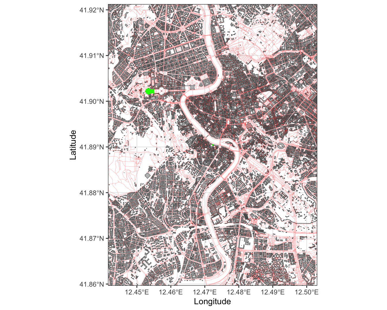
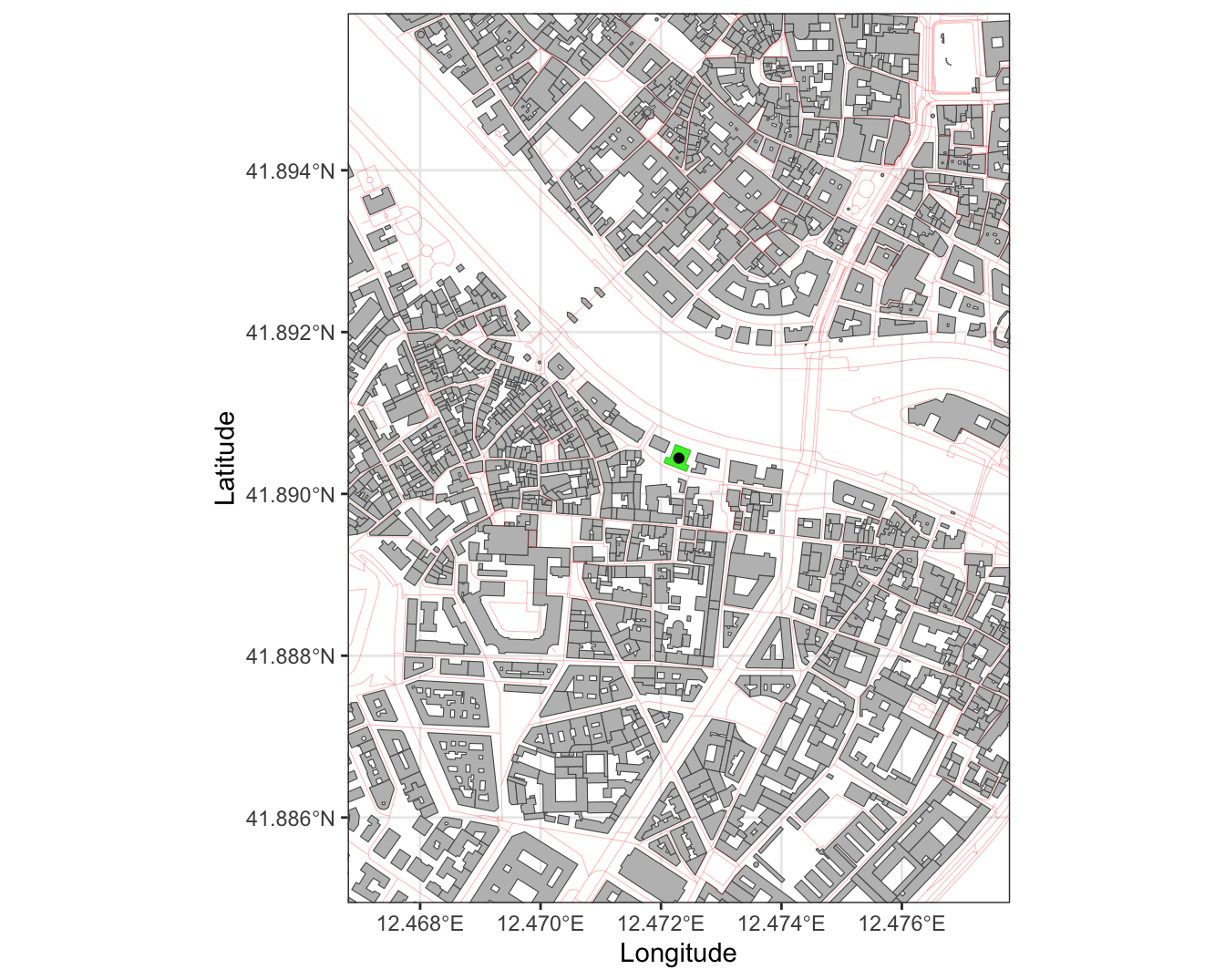
Finding the centroid of the JCU polygon and zooming out.

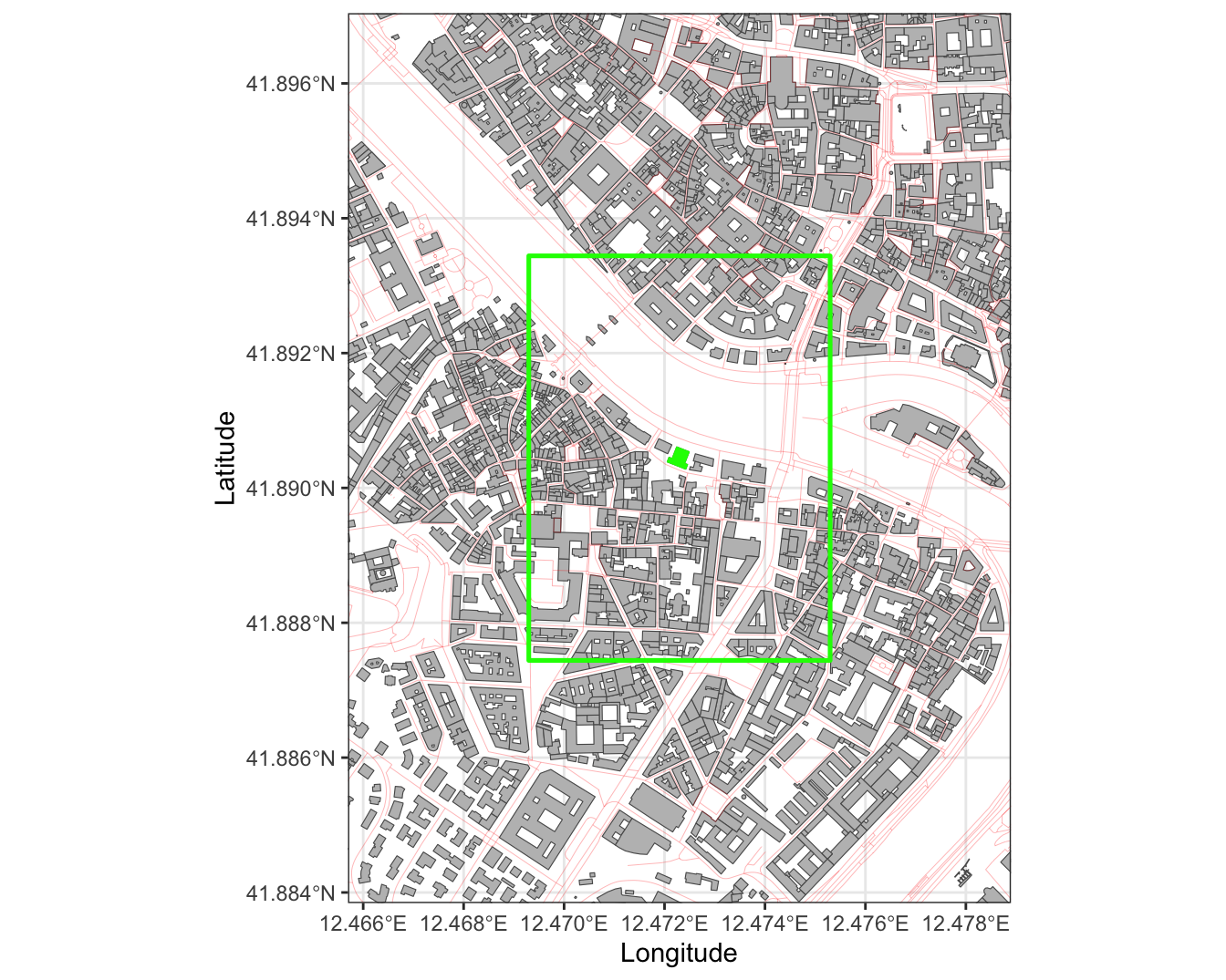
small_amount<-0.005

fig3<-ggplot()+
  geom_sf(data=gis_buildings, fill="grey")+
  geom_sf(data=gis_osm_roads, linewidth = 0.1, color = "red", alpha=0.5)+
  geom_sf(data=jcu, linewidth = 0.1, color = "green", fill = "green", alpha=0.8)+
  geom_point(data = jcu, x = jcu$lon_x, y= jcu$lat_y)+
  theme(legend.position="left")+
  theme_bw()+
  coord_sf(xlim = c(jcu$lon_x-small_amount, jcu$lon_x+small_amount), 
          ylim = c(jcu$lat_y-small_amount, jcu$lat_y+small_amount))+
  labs(x = "Longitude", y="Latitude")

Step3: Identify Relevant Points of Interest

Finding the centroid of the JCU polygon and zooming out.

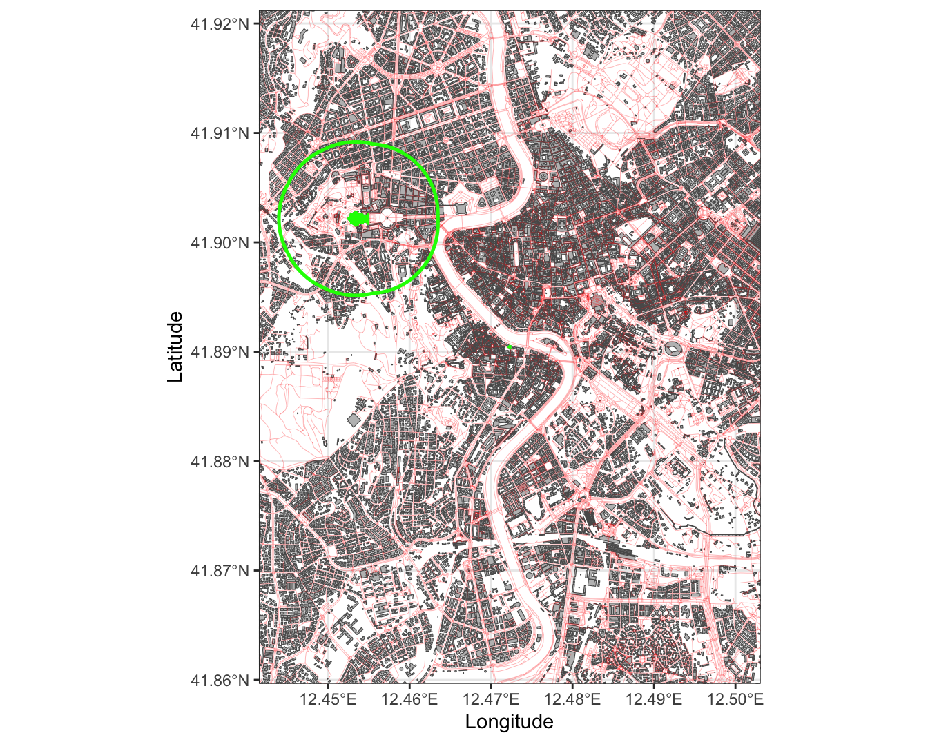
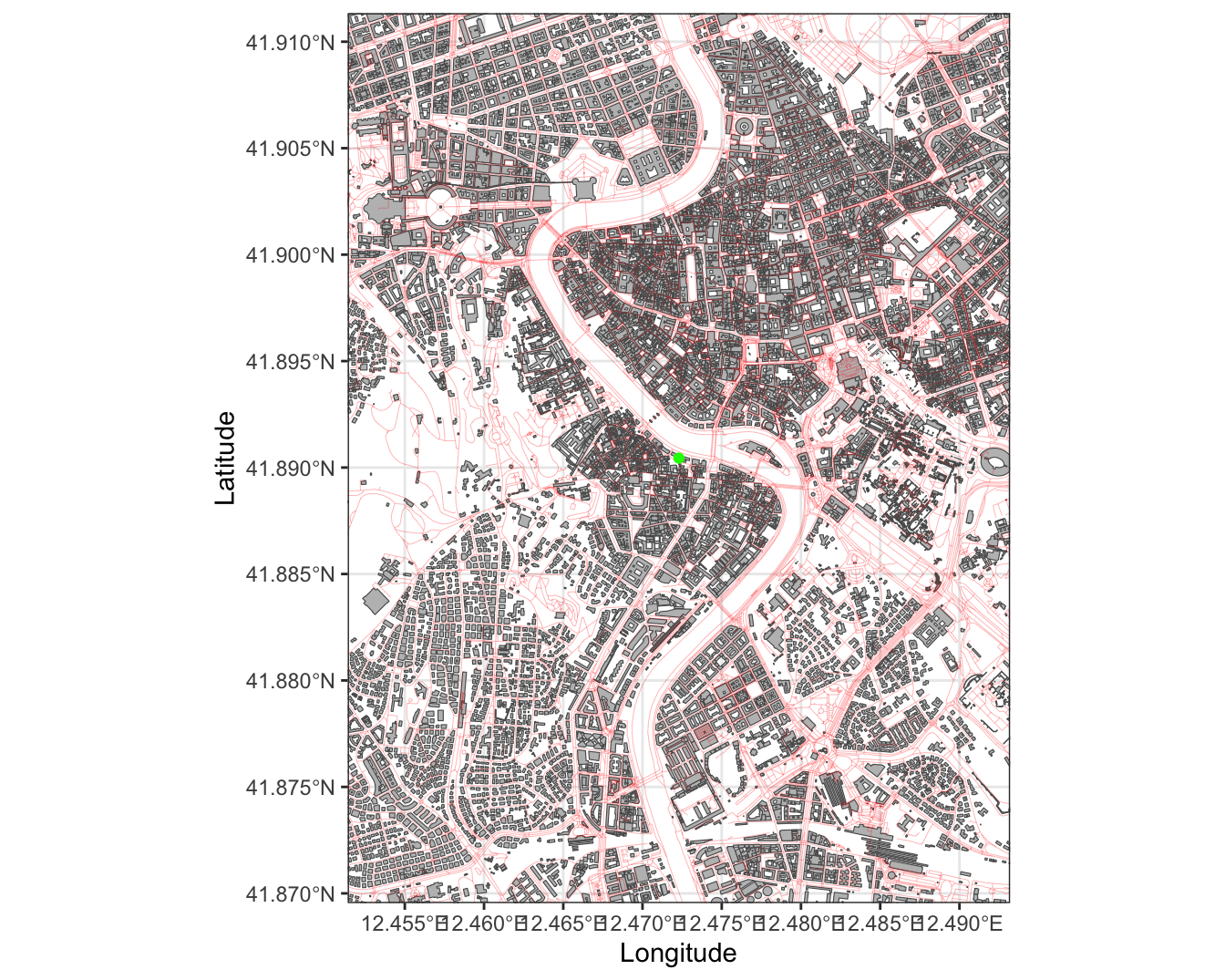
Step3: Identify Relevant Points of Interest

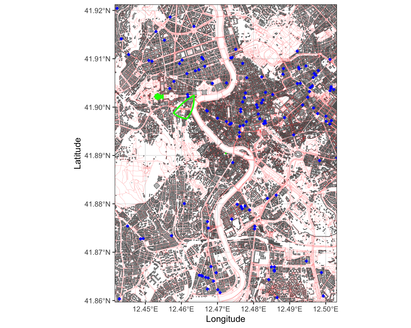
Finding the centroid of the JCU polygon and zooming out more.

small_amount<-0.019

fig4<-ggplot()+
  geom_sf(data=gis_buildings, fill="grey")+
  geom_sf(data=gis_osm_roads, linewidth = 0.1, color = "red", alpha=0.5)+
  geom_sf(data=jcu, linewidth = 0.1, color = "green", fill = "green", alpha=0.8)+
  geom_point(data = jcu, x = jcu$lon_x, y= jcu$lat_y, color = "green")+
  theme(legend.position="left")+
  theme_bw()+
  coord_sf(xlim = c(jcu$lon_x-small_amount, jcu$lon_x+small_amount), 
           ylim = c(jcu$lat_y-small_amount, jcu$lat_y+small_amount))+
  labs(x = "Longitude", y="Latitude")

Step3: Identify Relevant Points of Interest

Finding the centroid of the JCU polygon and zooming out more.

Step3: Identify Relevant Points of Interest

We know from the student’s specifications that they are interested in:

• living 1.5km (0.93 miles) away from JCU.

• living 0.7km (0.43 miles) away from the Vatican.

• living 0.5km (0.31 miles) from a bank.

We now need to identify the additional points of interest:

• Vatican
• banks

Step3: Identify Relevant Points of Interest

To identify the other points of interest, we proceed the same way we proceeded the same way we did with JCU.

Thus, we can now subset our dataframes.

vatican <- subset(gis_osm_pofw, name=="Basilica di San Pietro")
banks <- subset(gis_osm_pois, fclass=="bank")

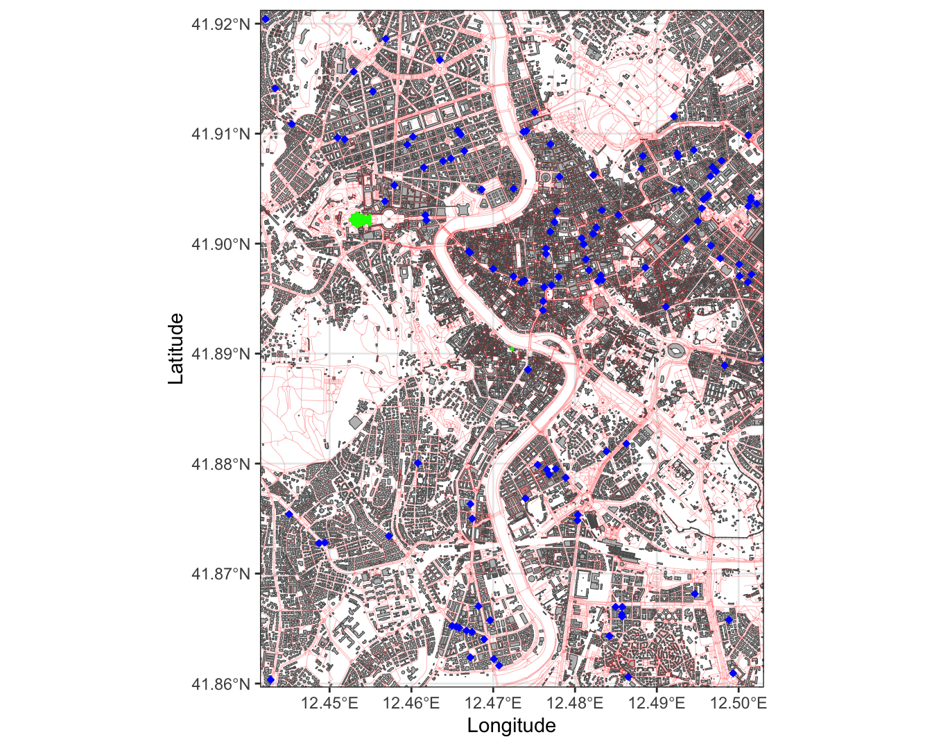
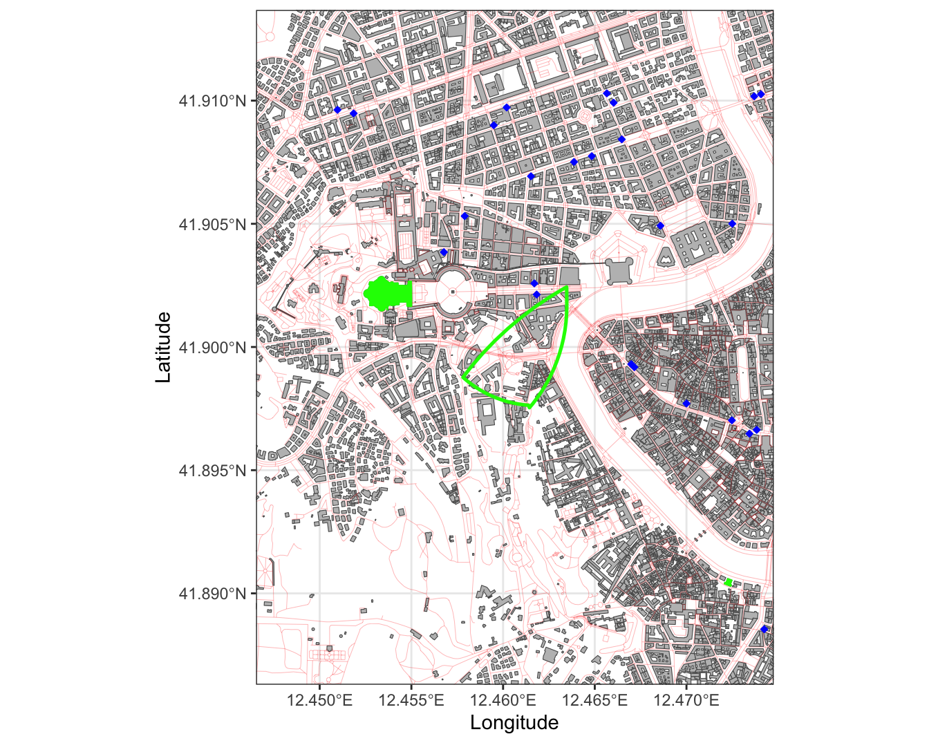
Step3: Identify Relevant Points of Interest

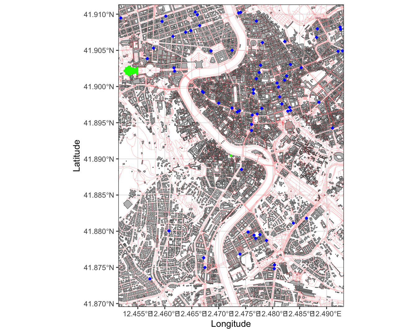
Let us now map the three points of interest on our map

small_amount<-0.019
fig5<-ggplot()+
  geom_sf(data=gis_buildings, fill="grey")+
  geom_sf(data=gis_osm_roads, linewidth = 0.1, color = "red", alpha=0.5)+
  geom_sf(data = jcu, fill="green", color = "green")+
  geom_sf(data = vatican, fill="green", color = "green")+
  geom_sf(data = banks, shape=23, fill="blue", color="blue", size=1)+
  theme(legend.position="left")+
  theme_bw()+
  coord_sf(xlim = c(jcu$lon_x-small_amount, jcu$lon_x+small_amount), 
          ylim = c(jcu$lat_y-small_amount, jcu$lat_y+small_amount))+
  labs(x = "Longitude", y="Latitude")

Step3: Identify Relevant Points of Interest

Let us now map the three points of interest on our map

Step3: Identify Relevant Points of Interest

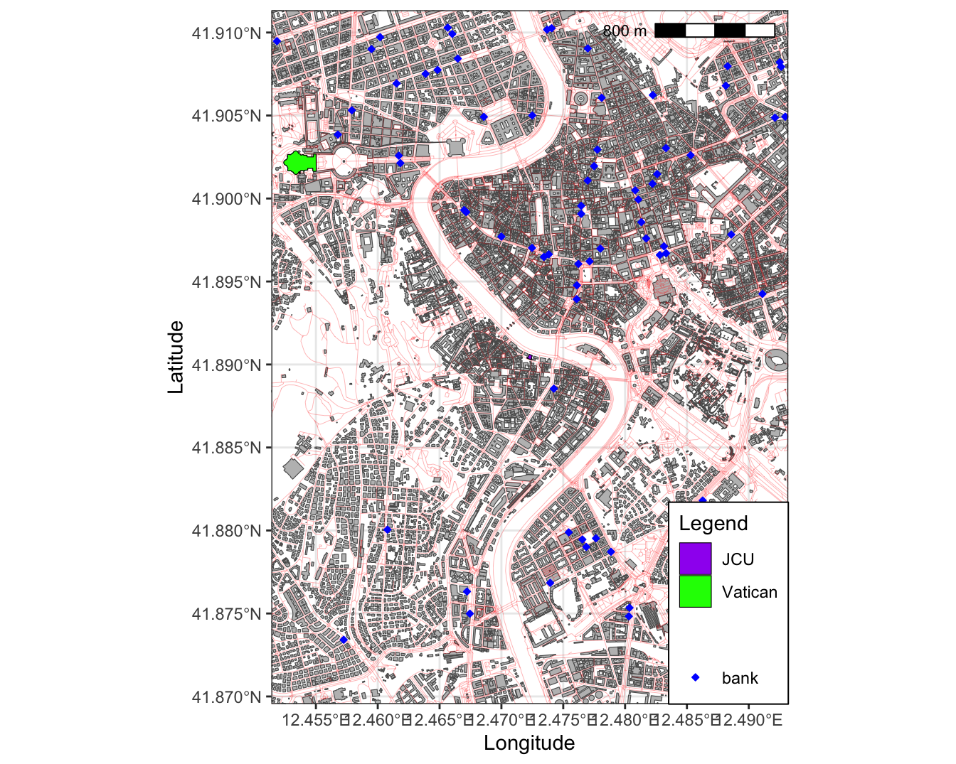
Let us also add a legend for better visibility for the points of interest

To do that we need to combine the shape of the same type on one dataframe

• The Vatican and JCU
• The Banks

Step3: Identify Relevant Points of Interest

#Step1: Selecting one colum so that we can bind the files
vatican1<-subset(vatican, select = c(name))
jcu1<-subset(jcu, select = c(name))
jcu_and_vatican<-rbind(vatican1, jcu1)

Step3: Identify Relevant Points of Interest

#Step2: Checking if the names of that will appear in legend may be too long
jcu_and_vatican$name

[1] "Basilica di San Pietro"              
[2] "John Cabot University - Tiber Campus"

You can see that we can change the two names for a more elegant legend

• “Basilica di San Pietro” = “Vatican”
• “John Cabot University - Tiber Campus” = “JCU”

Step3: Identify Relevant Points of Interest

#Step2: Checking if the names of that will appear in legend may be too long
jcu_and_vatican$name[jcu_and_vatican$name=="Basilica di San Pietro"]<-"Vatican"
jcu_and_vatican$name[jcu_and_vatican$name=="John Cabot University - Tiber Campus"]<-"JCU"

#Step3: Checking if the changes were made
jcu_and_vatican$name

[1] "Vatican" "JCU"    

Step3: Identify Relevant Points of Interest

small_amount<-0.019
fig6<-ggplot()+
  geom_sf(data=gis_buildings, fill="grey")+
  geom_sf(data=gis_osm_roads, linewidth = 0.1, color = "red", alpha=0.5)+
  geom_sf(data = jcu_and_vatican,  
          aes(fill = name), color = "black")+
  scale_fill_manual(name = "Legend", 
                    values=c("purple", "green"),
                    guide = guide_legend(order = 1))+
  geom_sf(data = banks,
          aes(color = fclass),
          fill="blue",
          size=1, 
          shape = 23) +
  scale_color_manual(name = "", 
                    values=c("blue"),
                    guide = guide_legend(order = 2))+
  theme(legend.position="left")+
  theme_bw()+
  coord_sf(xlim = c(jcu$lon_x-small_amount, jcu$lon_x+small_amount), 
           ylim = c(jcu$lat_y-small_amount, jcu$lat_y+small_amount))+
  labs(x = "Longitude", y="Latitude")+
    theme(
        legend.justification = c(1, 0), 
        legend.position = c(1, 0),
        #Legend.position values should be between 0 and 1. c(0,0) corresponds to the "bottom left"
        #and c(1,1) corresponds to the "top right" position.
        legend.spacing.y = unit(0.05, 'cm'),
        legend.box.background = element_rect(fill='white'),
        legend.background = element_blank())+
ggspatial::annotation_scale(location = 'tr')

Step3: Identify Relevant Points of Interest

Step4: Create Buffers

We know that Mark wants a place with the following specifications:

• living 1.5km (0.93 miles) away from JCU.

• living 0.7km (0.43 miles) away from the Vatican.

• living 0.5km (0.31 miles) from a bank.

We want to create buffers from the main points of interest

Step4: Create Buffers

A buffer in GIS is a reclassification based on distance: classification of within/without a given proximity.

Before we create a buffer, we want to see our unit of measurement

st_crs(jcu)

Coordinate Reference System:
  User input: WGS 84 
  wkt:
GEOGCRS["WGS 84",
    ENSEMBLE["World Geodetic System 1984 ensemble",
        MEMBER["World Geodetic System 1984 (Transit)"],
        MEMBER["World Geodetic System 1984 (G730)"],
        MEMBER["World Geodetic System 1984 (G873)"],
        MEMBER["World Geodetic System 1984 (G1150)"],
        MEMBER["World Geodetic System 1984 (G1674)"],
        MEMBER["World Geodetic System 1984 (G1762)"],
        MEMBER["World Geodetic System 1984 (G2139)"],
        MEMBER["World Geodetic System 1984 (G2296)"],
        ELLIPSOID["WGS 84",6378137,298.257223563,
            LENGTHUNIT["metre",1]],
        ENSEMBLEACCURACY[2.0]],
    PRIMEM["Greenwich",0,
        ANGLEUNIT["degree",0.0174532925199433]],
    CS[ellipsoidal,2],
        AXIS["geodetic latitude (Lat)",north,
            ORDER[1],
            ANGLEUNIT["degree",0.0174532925199433]],
        AXIS["geodetic longitude (Lon)",east,
            ORDER[2],
            ANGLEUNIT["degree",0.0174532925199433]],
    USAGE[
        SCOPE["Horizontal component of 3D system."],
        AREA["World."],
        BBOX[-90,-180,90,180]],
    ID["EPSG",4326]]

Step4: Create Buffers

We see that within CS[ellipsoidal,2] that the unit is “degree”

Before we calculate those buffers, we need to have metric units

We can do that easily by reprojecting our shapefiles

We accomplish that by simply using:

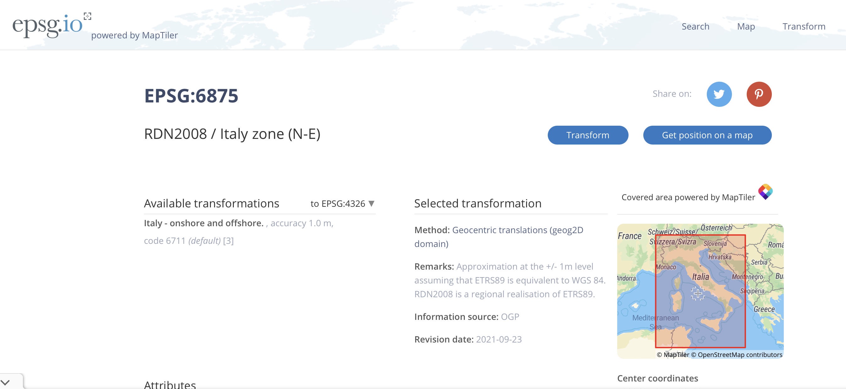
#Step1: Turning the relevant shape to a metric systems
jcu_reproj = st_transform(jcu, 6875)

Step4: Create Buffers

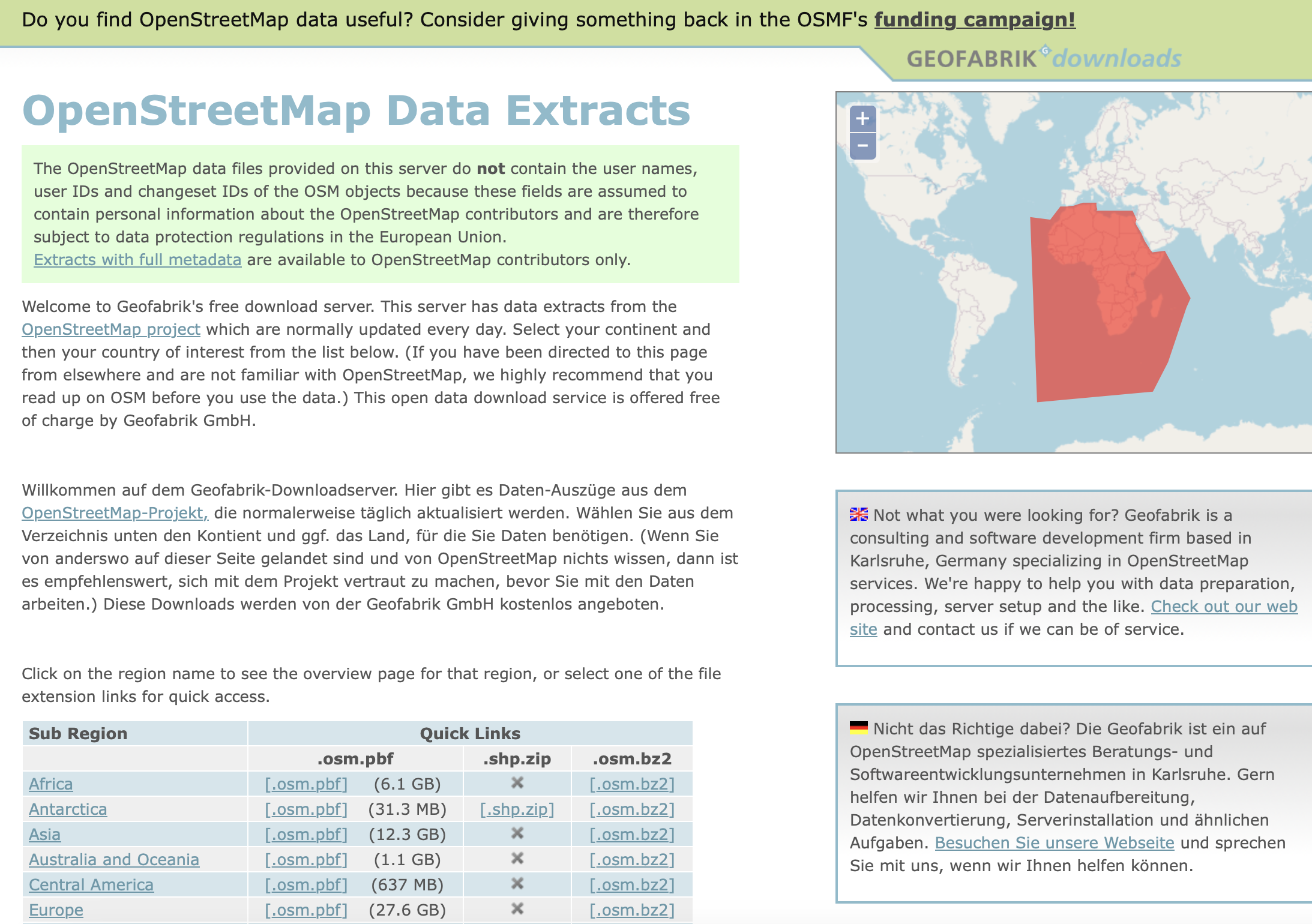
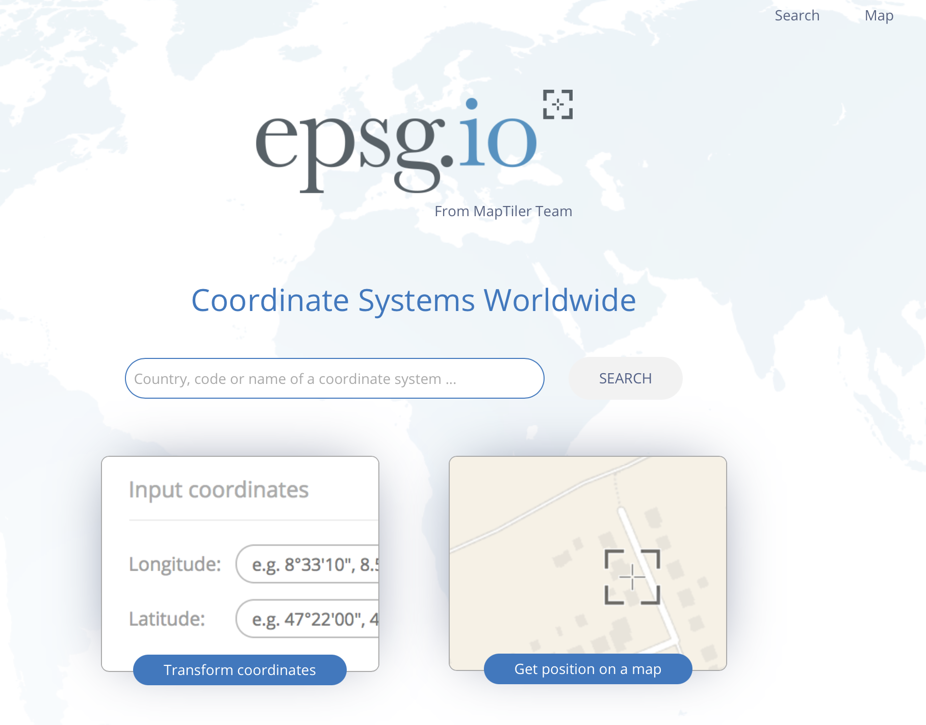
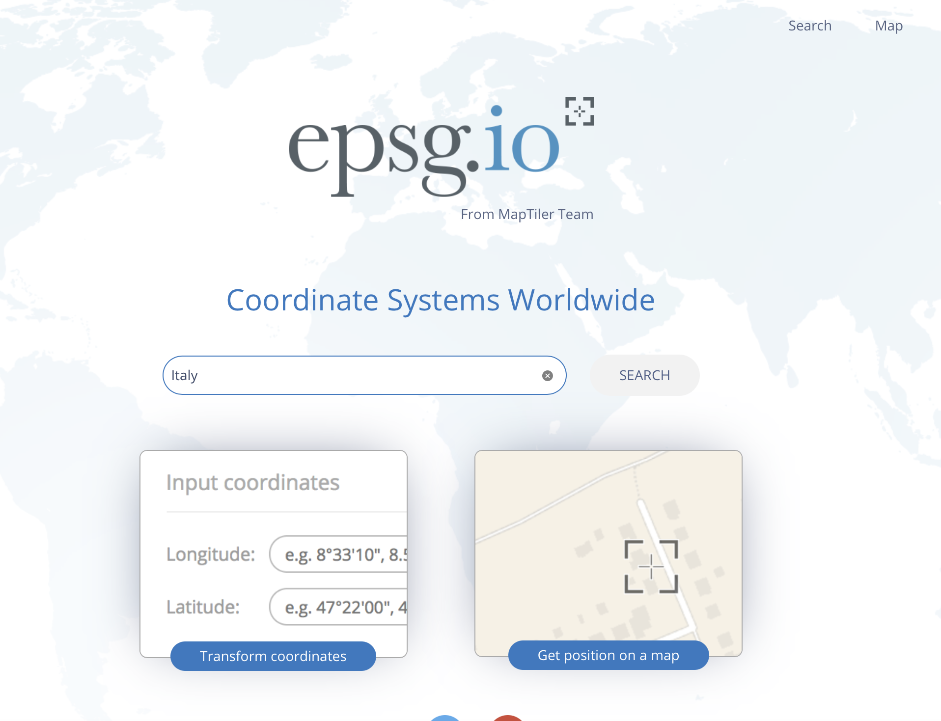
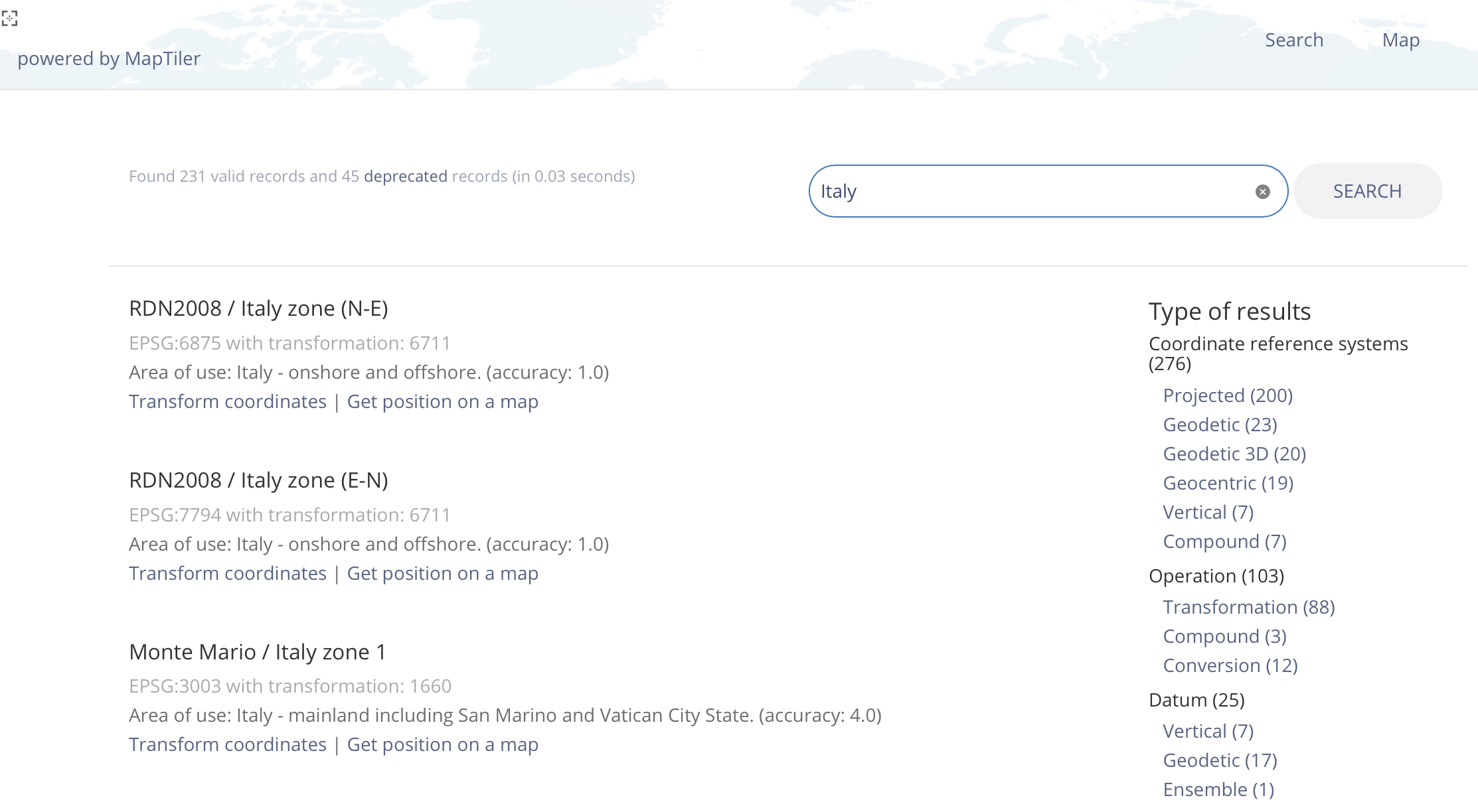
The natural question is where does 6875 come from?

This is from https://epsg.io

EPSG Geodetic Parameter Dataset is a public registry of geodetic datums, spatial reference systems.

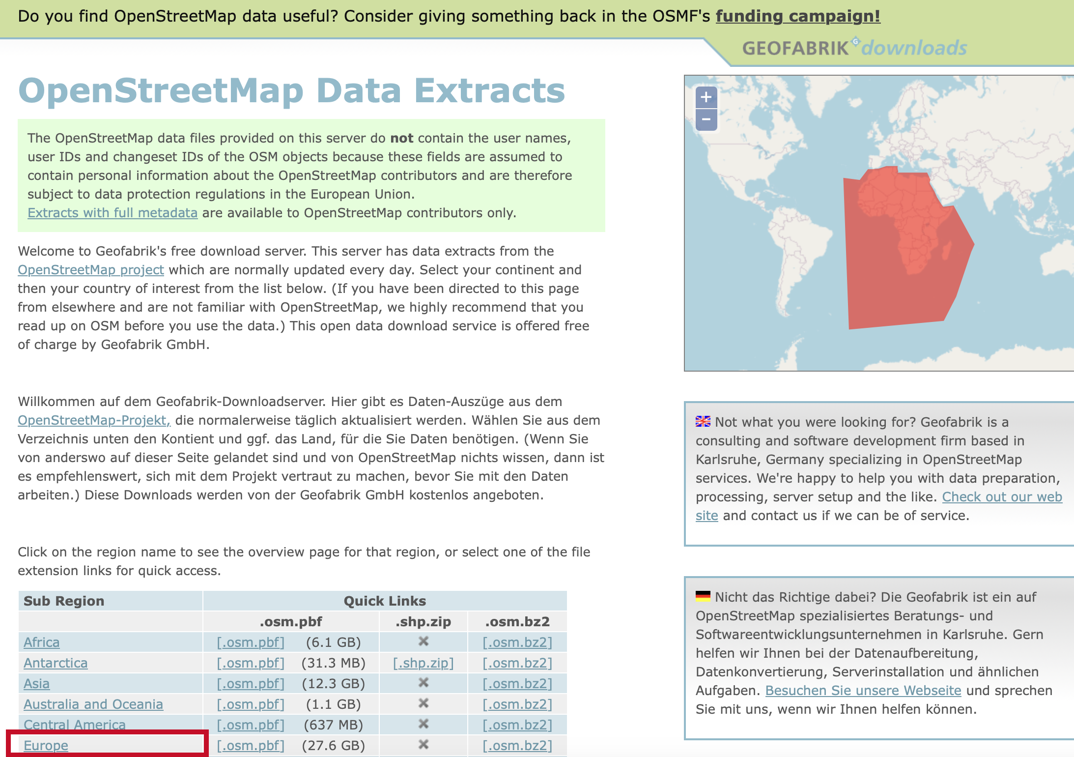
Step4: Create Buffers

Step4: Create Buffers

Step4: Create Buffers

Step4: Create Buffers

Step4: Create Buffers

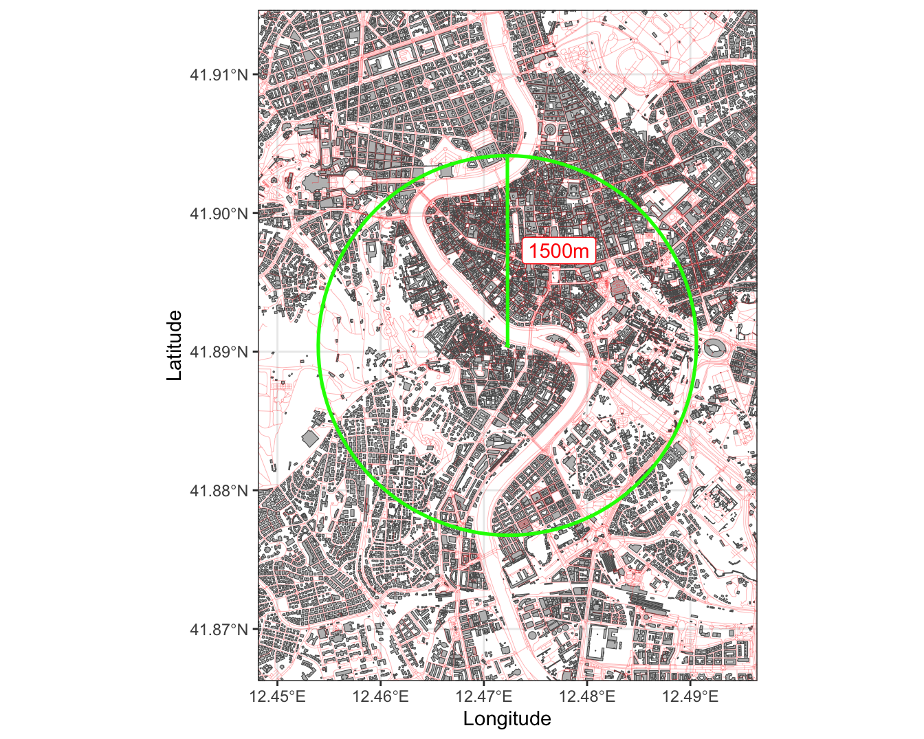
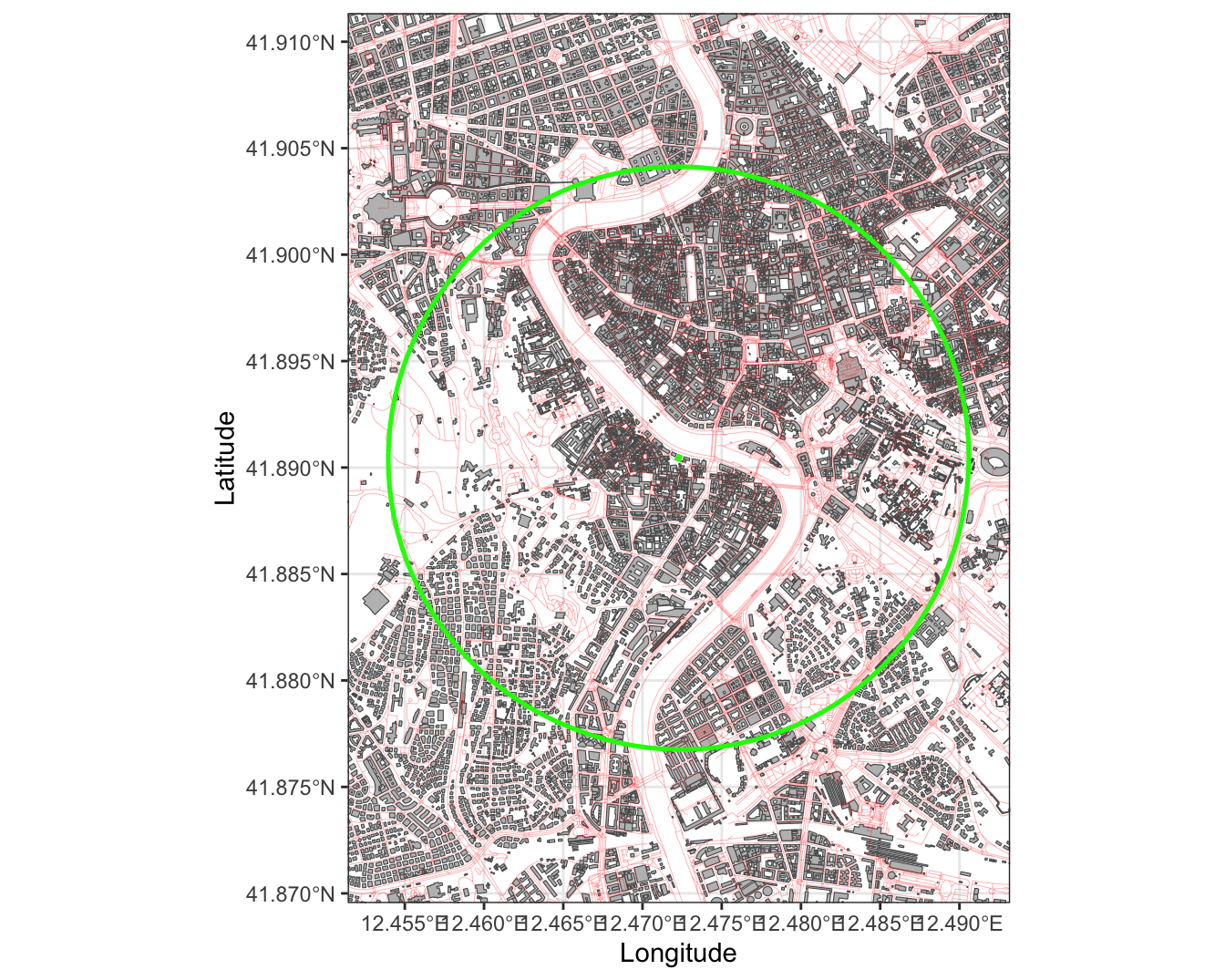
#Step1: Turning the relevant shape to a metric systems
jcu_reproj = st_transform(jcu, 6875)
#Step2: Creating the 1500m 
jcu_buff <- st_buffer(jcu_reproj, dist = 1500)
#Step3: Turning back to WGS84
jcu_buff2<-st_transform(st_as_sf(jcu_buff), st_crs(jcu))

Step4: Create Buffers

small_amount<-0.019
fig4<-ggplot()+
  geom_sf(data=gis_buildings, fill="grey")+
  geom_sf(data=gis_osm_roads, linewidth = 0.1, color = "red", alpha=0.5)+
  geom_sf(data = jcu, fill="green", color = "green")+
  geom_sf(data = jcu_buff2, fill=NA, color = "green", linewidth = 0.9)+
  theme(legend.position="left")+
  theme_bw()+
  coord_sf(xlim = c(jcu$lon_x-small_amount, jcu$lon_x+small_amount), 
           ylim = c(jcu$lat_y-small_amount, jcu$lat_y+small_amount))+
  labs(x = "Longitude", y="Latitude")

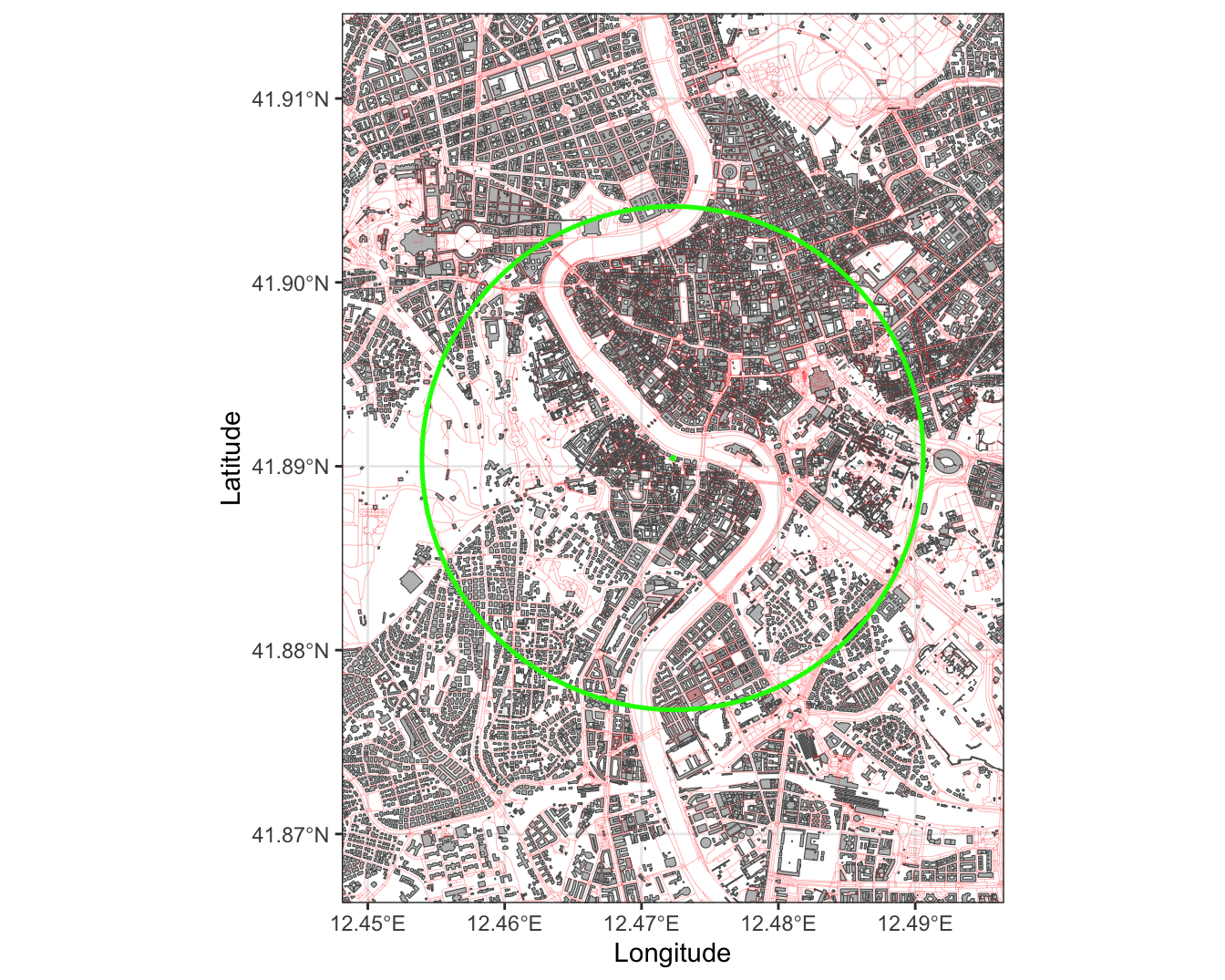
Step4: Create Buffers

Step4: Create Buffers

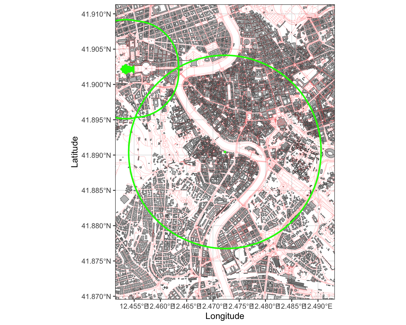
We now repeat the same procedure for the Vatican

#Creating the 700m buffer
#Step1: Turning the relevant shape to a metric systems
vatican_reproj = st_transform(vatican, 6875)
#Step2: Creating the 700m 
vatican_buff <- st_buffer(vatican_reproj, dist = 700)
#Step3: Turning back to WGS84
vatican_buff2<-st_transform(st_as_sf(vatican_buff), st_crs(jcu))

Step4: Create Buffers

small_amount<-0.019
fig5<-ggplot()+
  geom_sf(data=gis_buildings, fill="grey")+
  geom_sf(data=gis_osm_roads, linewidth = 0.1, color = "red", alpha=0.5)+
  geom_sf(data = jcu, fill="green", color = "green")+
  geom_sf(data = jcu_buff2, fill=NA, color = "green", linewidth = 0.9)+
  geom_sf(data = vatican, fill="green", color = "green")+
  geom_sf(data = vatican_buff2, fill=NA, color = "green", linewidth = 0.9)+
  theme(legend.position="left")+
  theme_bw()+
  coord_sf(xlim = c(jcu$lon_x-small_amount, jcu$lon_x+small_amount), 
           ylim = c(jcu$lat_y-small_amount, jcu$lat_y+small_amount))+
  labs(x = "Longitude", y="Latitude")

Step4: Create Buffers

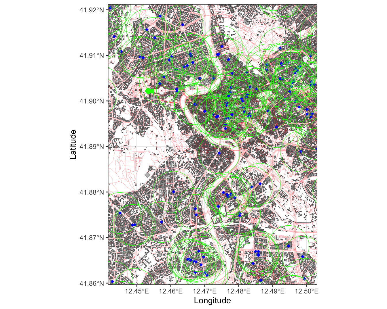
Step4: Create Buffers

We now repeat the same procedure for the banks

#Creating the 500m buffer
#Step1: Turning the relevant shape to a metric systems
banks_reproj = st_transform(banks, 6875)
#Step2: Creating the 700m 
banks_buff <- st_buffer(banks_reproj, dist = 500)
#Step3: Turning back to WGS84
banks_buff2<-st_transform(st_as_sf(banks_buff), st_crs(jcu))

Step4: Create Buffers

small_amount<-0.019

fig6<-ggplot()+
  geom_sf(data=gis_buildings, fill="grey")+
  geom_sf(data=gis_osm_roads, linewidth = 0.1, color = "red", alpha=0.5)+
  geom_sf(data = jcu, fill="green", color = "green")+
  geom_sf(data = jcu_buff2, fill=NA, color = "green", linewidth = 0.9)+
  geom_sf(data = vatican, fill="green", color = "green")+
  geom_sf(data = vatican_buff2, fill=NA, color = "green", linewidth = 0.9)+
  geom_sf(data = banks, fill="green", color = "green")+
  geom_sf(data = banks_buff2, fill=NA, color = "green", linewidth = 0.9)+
  theme(legend.position="left")+
  theme_bw()+
  coord_sf(xlim = c(jcu$lon_x-small_amount, jcu$lon_x+small_amount), 
           ylim = c(jcu$lat_y-small_amount, jcu$lat_y+small_amount))+
  labs(x = "Longitude", y="Latitude")

Step4: Create Buffers

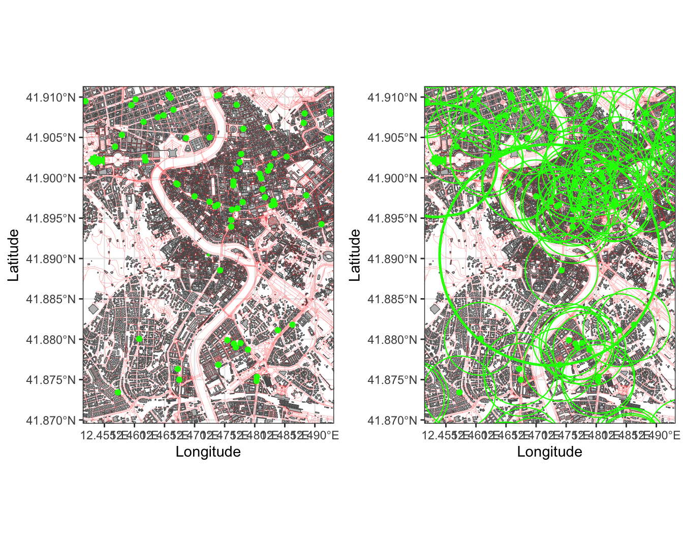
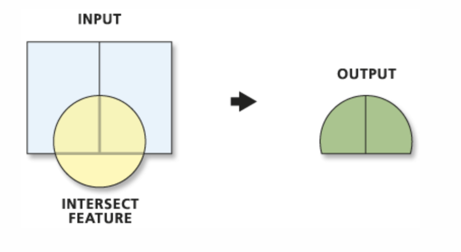
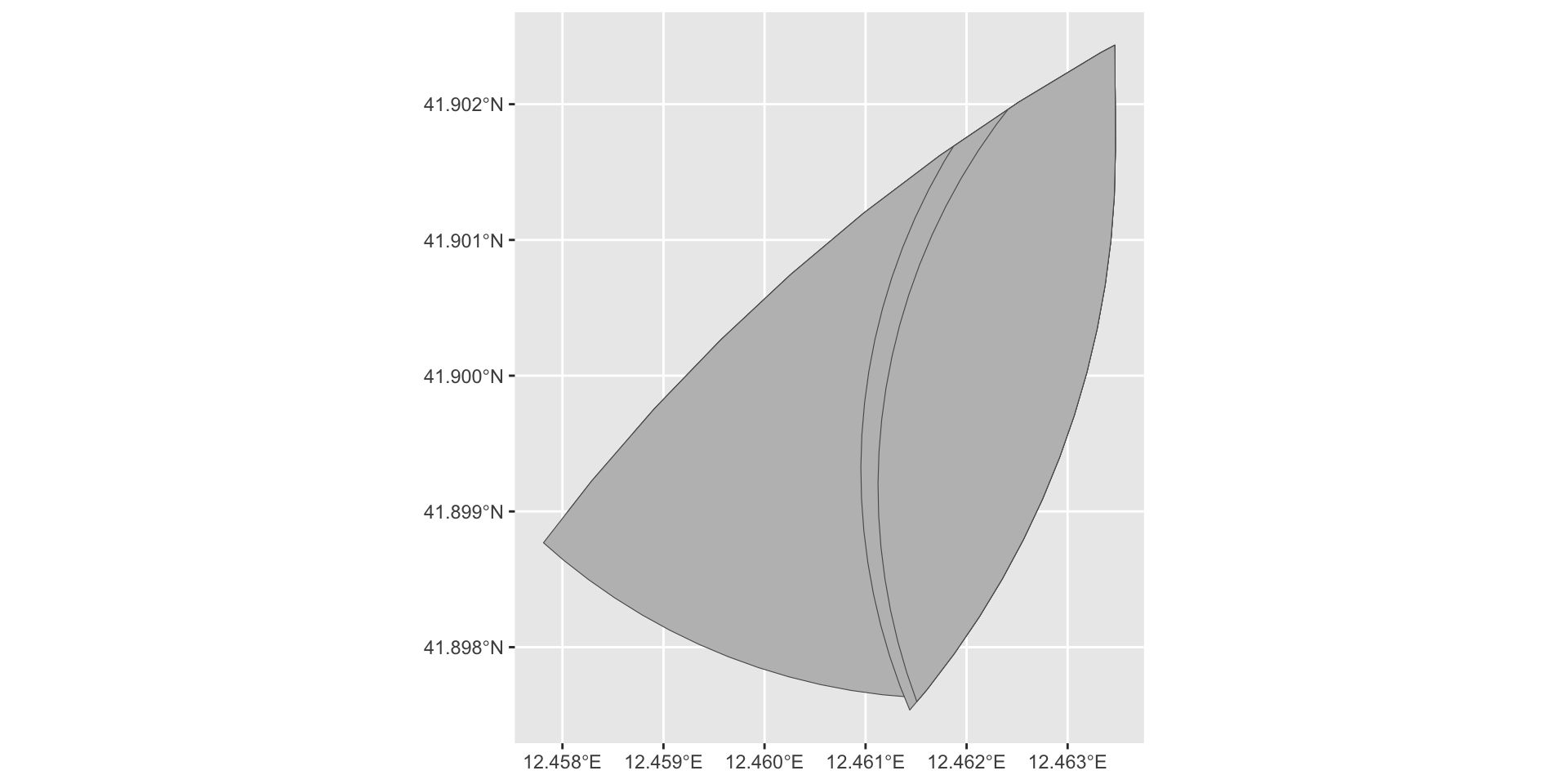
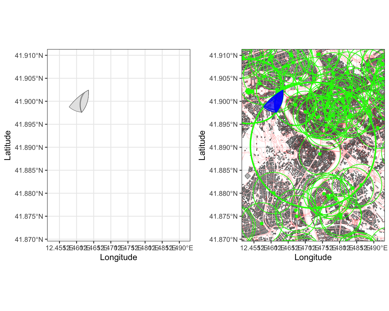
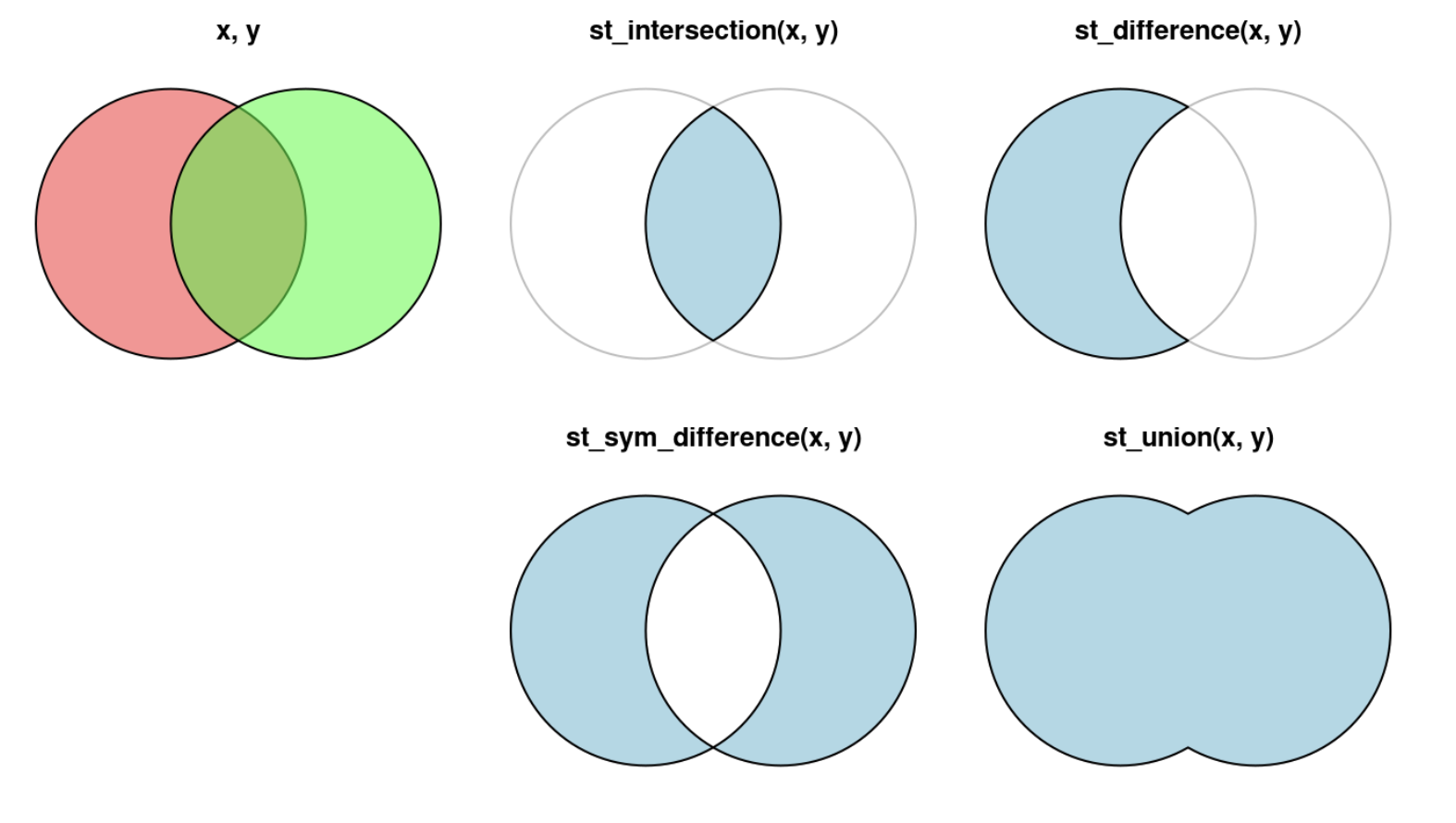
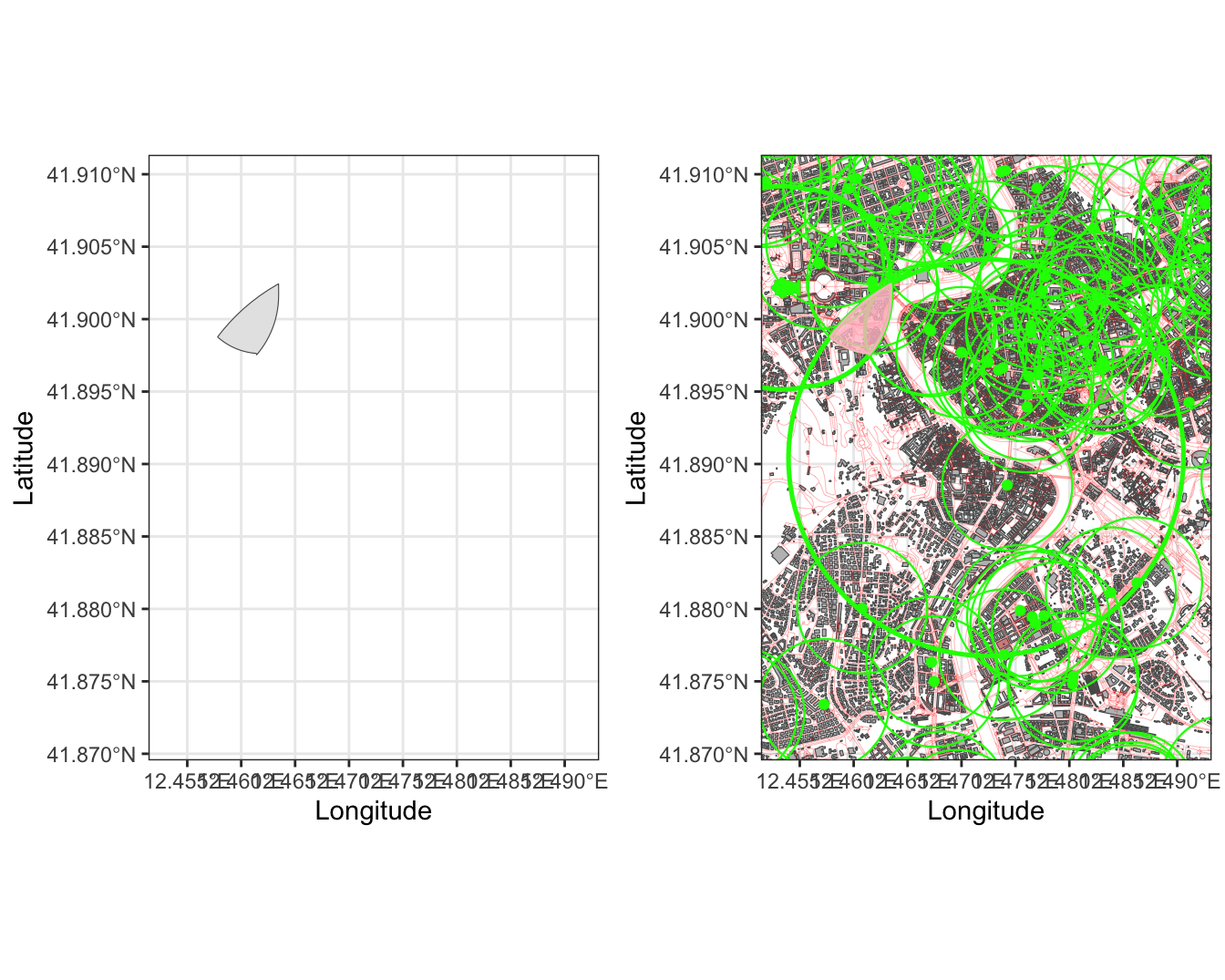
Step5: Intersecting the Buffers

Intersection computes a geometric intersection of the input features.

Step5: Intersecting the Buffers

#Intersecting the Buffers
sf_inters<-st_intersection(jcu_buff2, vatican_buff2)

Step5: Intersecting the Buffers

Step5: Intersecting the Buffers

#Intersecting the Buffers
sf_inters2<-st_intersection(sf_inters, banks_buff2)

Step5: Intersecting the Buffers

Step5: Intersecting the Buffers

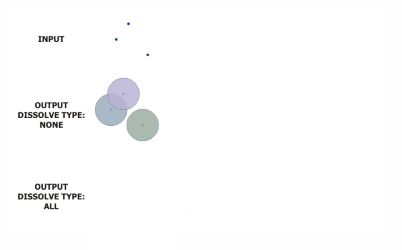
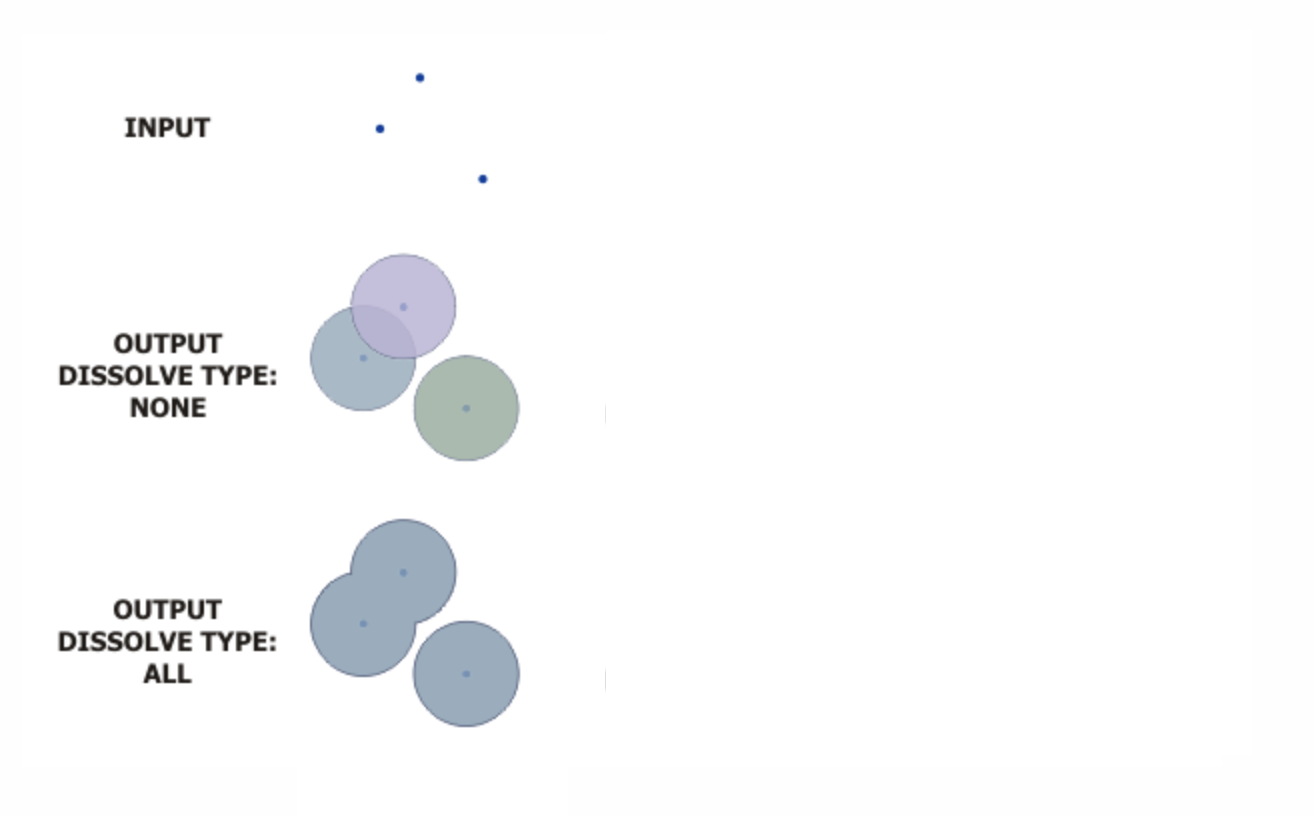
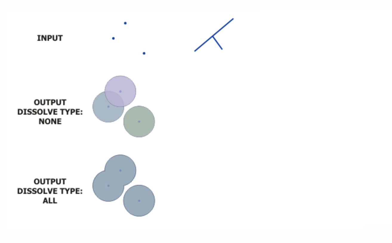
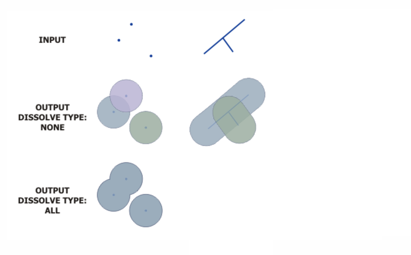
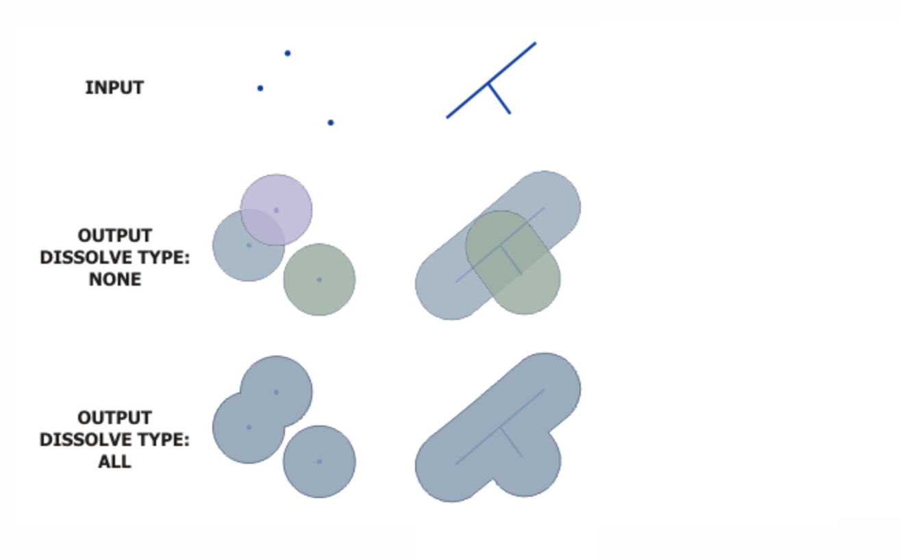
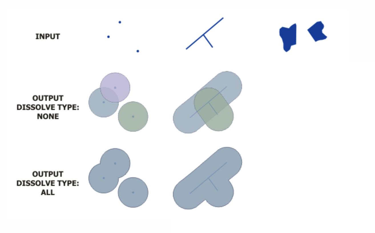
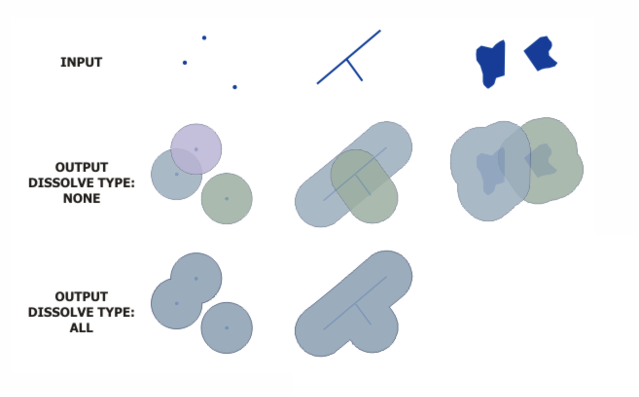
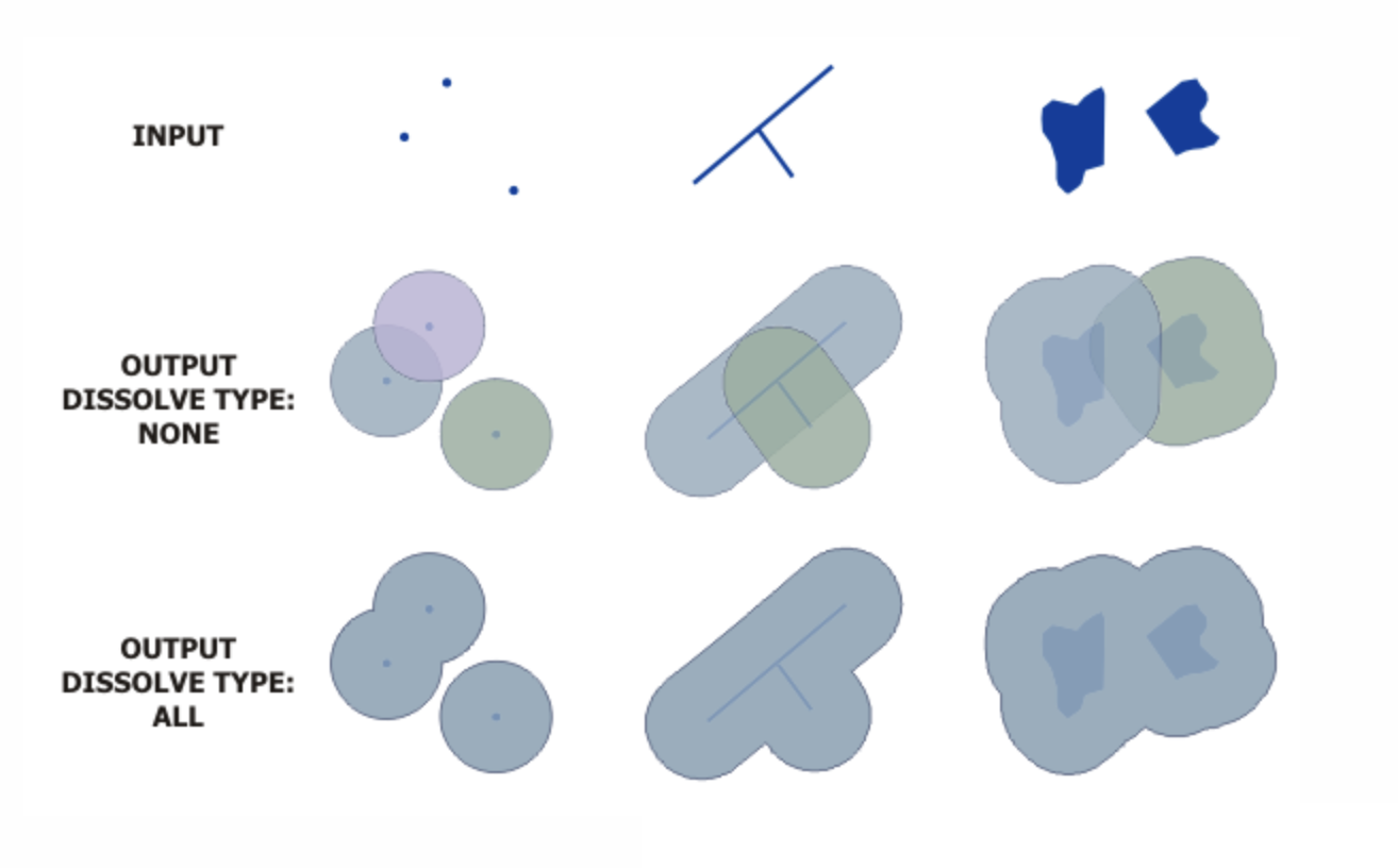
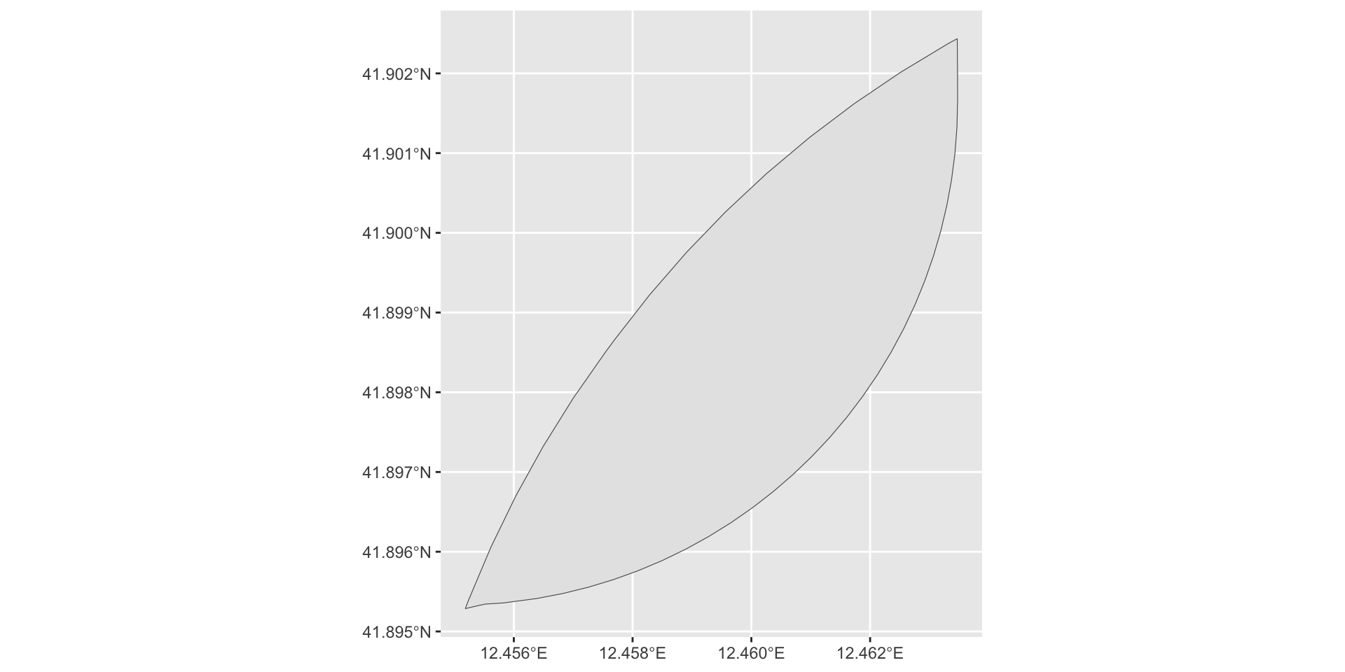
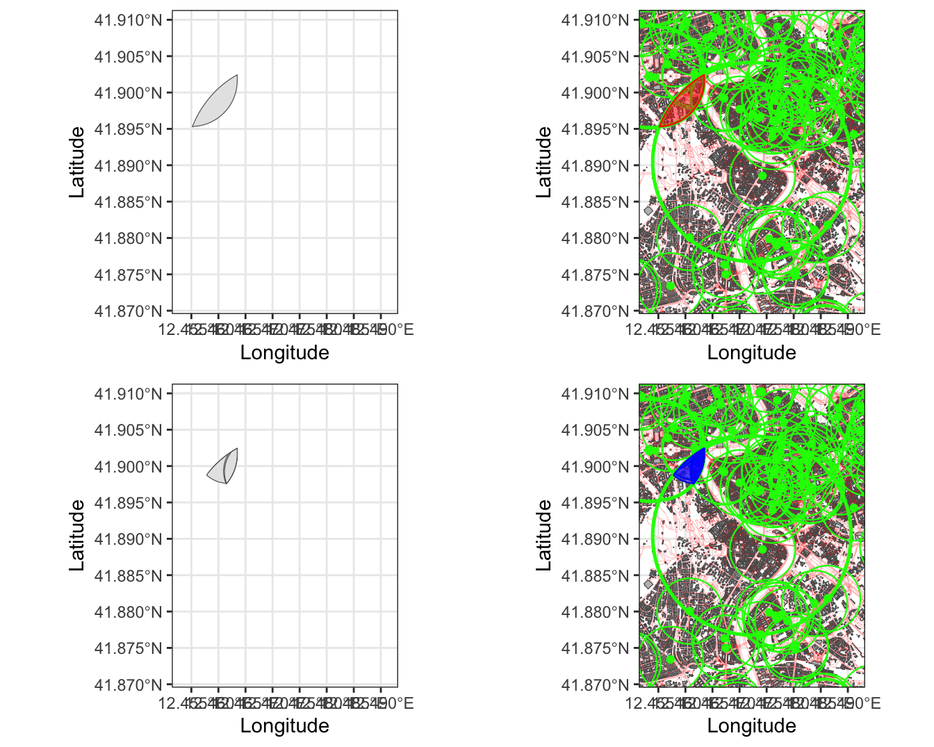
Step6: Performing Unions on Shapes

st_union takes two or more geometry columns and returns a geometry column

The output column contains the geometries that represent the spatial union of the geometries in each row of the input columns.

Step6: Performing Unions on Shapes

#Taking the Union
dissolve_sf <- st_union(sf_inters2)

Step6: Performing Unions on Shapes

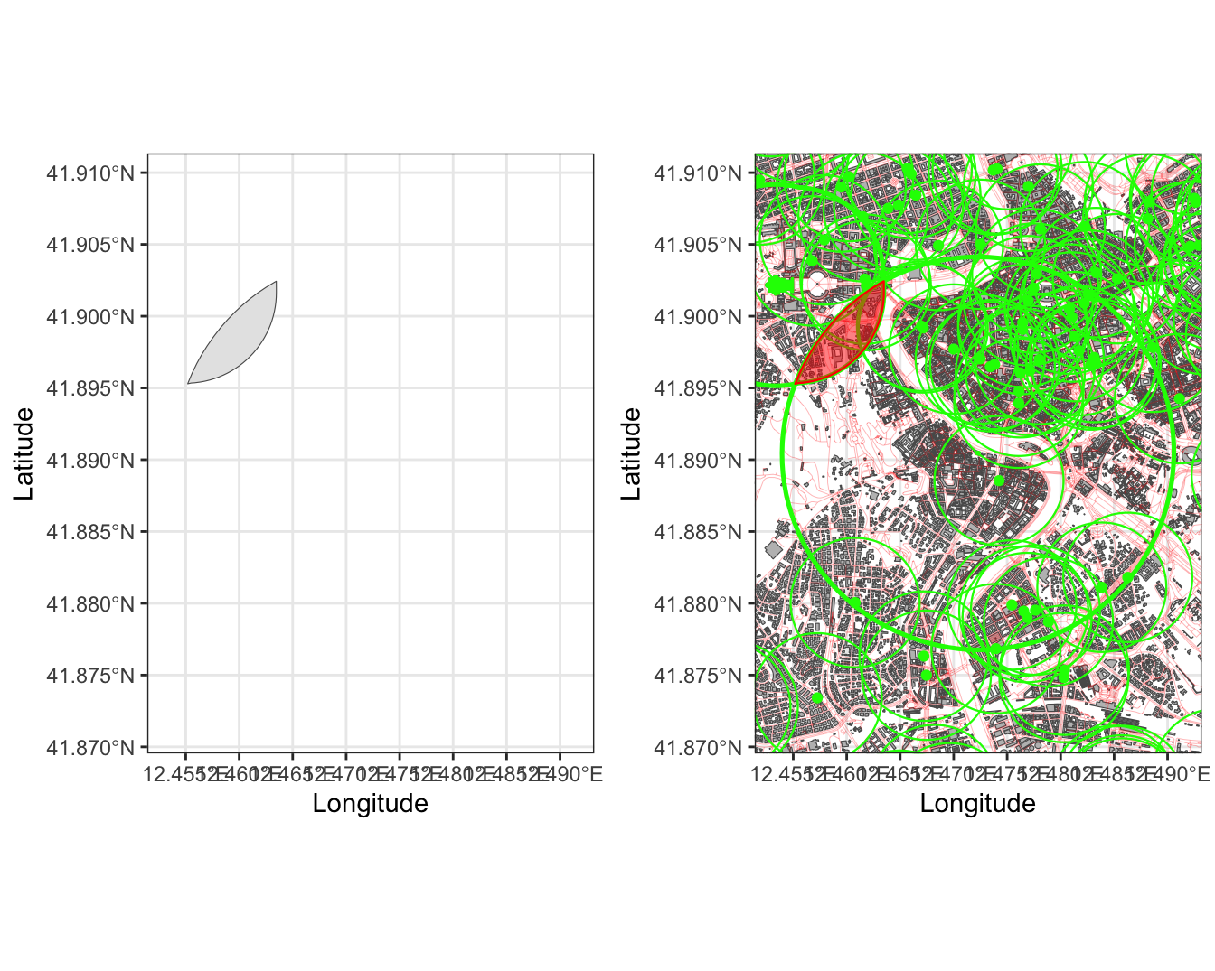
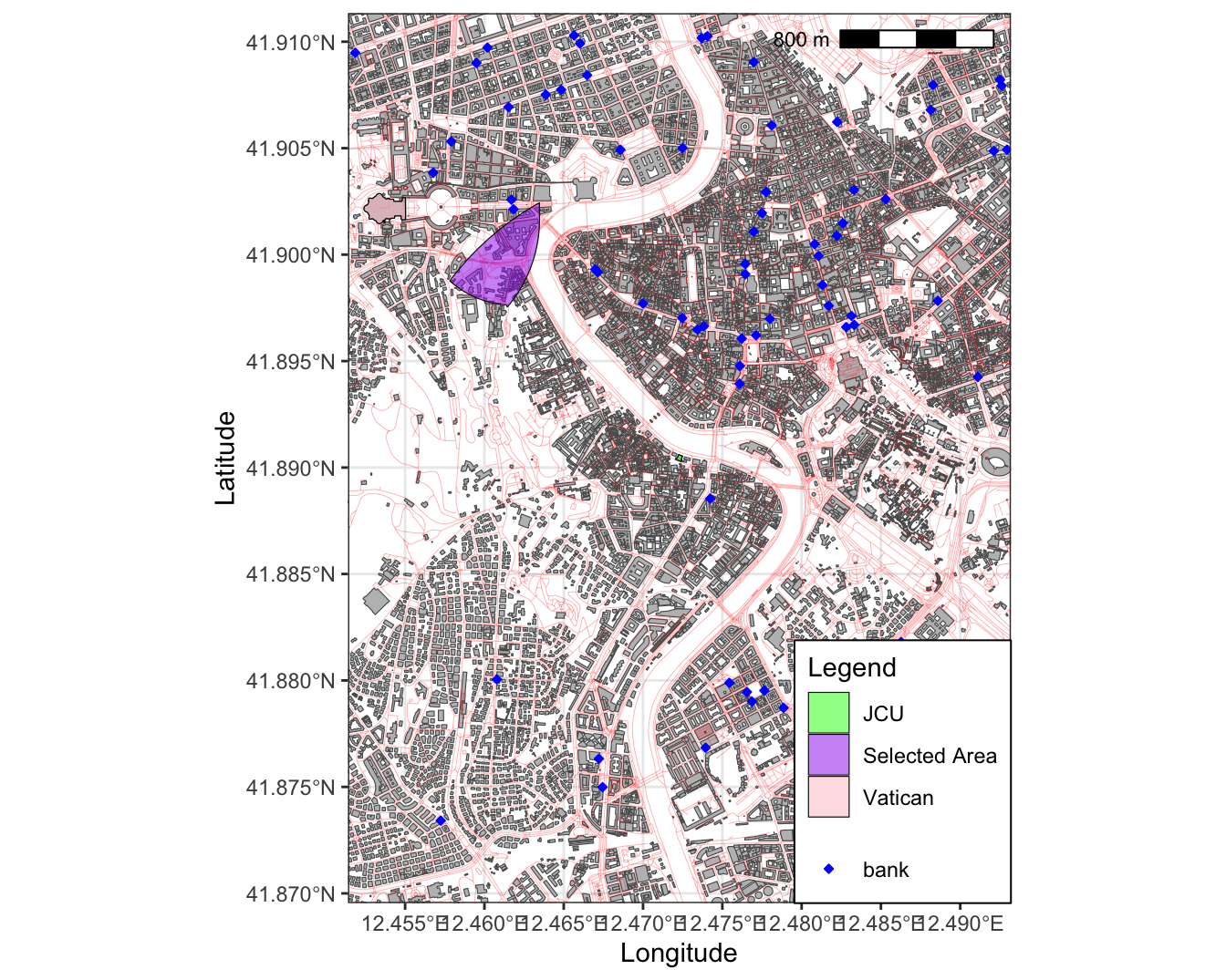
Creating a Map for Mark

The final step is to create a map for Mark that shows where he should live

• The base map

Creating a Map for Mark

The final step is to create a map for Mark that shows where he should live

• The base map

fig10

Creating a Map for Mark

The final step is to create a map for Mark that shows where he should live

• The base map
• Merging the relevant polygons

#Step1: Selecting one column so that we can bind the files
vatican1<-subset(vatican, select = c(name))
jcu1<-subset(jcu, select = c(name))
jcu_and_vatican<-rbind(vatican1, jcu1)
dissolve_sf1<-st_as_sf(dissolve_sf)
dissolve_sf1$name<-"Selected Area"
st_geometry(dissolve_sf1)<-"Shape"
final_shapes<-rbind(jcu_and_vatican, dissolve_sf1)
final_shapes$name[final_shapes$name=="Basilica di San Pietro"]<-"Vatican"
final_shapes$name[final_shapes$name=="John Cabot University - Tiber Campus"]<-"JCU"

Creating a Map for Mark

The final step is to create a map for Mark that shows where he should live

small_amount<-0.019

fig10<-ggplot()+
  geom_sf(data=gis_buildings, fill="grey")+
  geom_sf(data=gis_osm_roads, linewidth = 0.1, color = "red", alpha=0.5)+
  geom_sf(data = final_shapes,  aes(fill = name), color = "black", alpha=0.5)+
  scale_fill_manual(name = "Legend", 
                    values=c("Vatican"="pink",
                             "JCU" = "green",
                             "Selected Area" = "purple"),
                    guide = guide_legend(order = 1))+
  geom_sf(data = banks,
          aes(color = fclass),
          fill="blue",
          size=1, 
          shape = 23) +
  scale_color_manual(name = NULL, 
                    values=c("blue"),
                    guide = guide_legend(order = 2))+
  theme(legend.position="left")+
  theme_bw()+
  coord_sf(xlim = c(jcu$lon_x-small_amount, jcu$lon_x+small_amount), 
           ylim = c(jcu$lat_y-small_amount, jcu$lat_y+small_amount))+
  labs(x = "Longitude", y="Latitude")+
    theme(
        legend.justification = c(1, 0), 
        legend.position = c(1, 0),
        #Legend.position values should be between 0 and 1. c(0,0) corresponds to the "bottom left"
        #and c(1,1) corresponds to the "top right" position.
        legend.spacing.y = unit(0.05, 'cm'),
        legend.box.background = element_rect(fill='white'),
        legend.background = element_blank())+
  ggspatial::annotation_scale(location = 'tr')

Creating a Map for Mark

The final step is to create a map for Mark that shows where he should live

Conclusion

We have learned a varierty of GIS tools today

1. Using Open Street Maps
2. Calculating polygon centroids
3. Changing Coordinate Systems
4. Creating buffers
5. Uniting different shapes in one
6. Intersections
7. Unions